Linear Regression
A Brief Review
About me


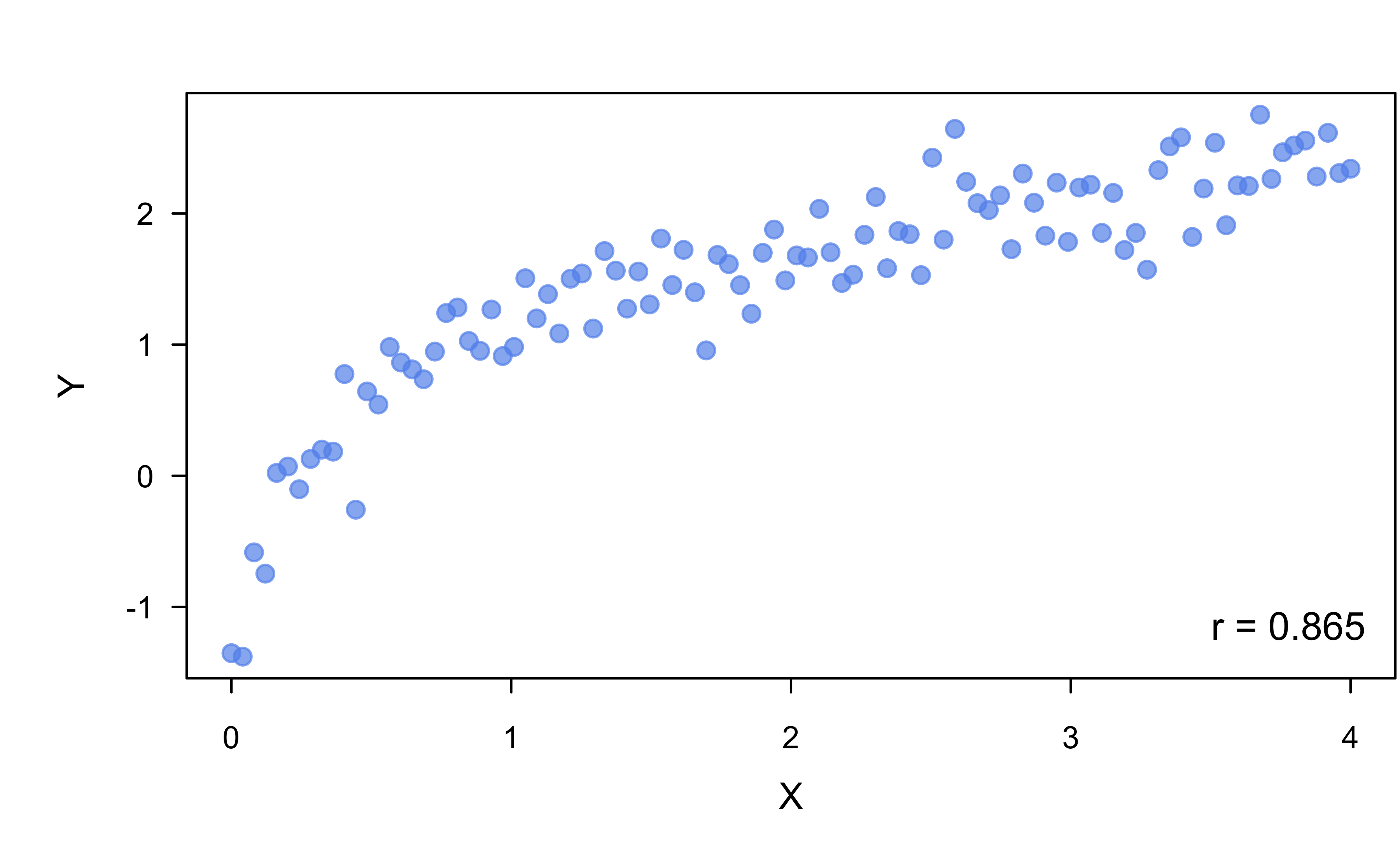
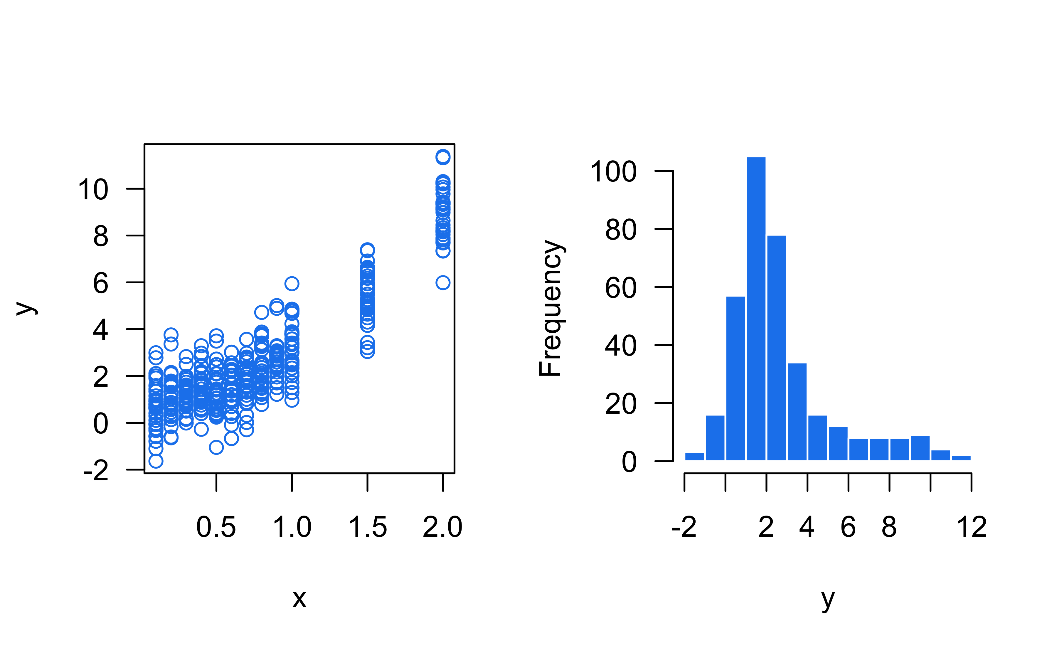
Statistical relationships
Show R code
# Simulate data from different SLR models
set.seed(101)  # for reproducibility
x <- seq(from = 0, to = 4, length = 100)
y <- cbind(
  1 + x + rnorm(length(x)),  # linear
  1 + (x - 2)^2 + rnorm(length(x)),  # quadratic
  1 + log(x + 0.1) + rnorm(length(x), sd = 0.3),  # logarithmic
  1 + rnorm(length(x))  # no association
)

# Scatterplot of X vs. each Y in a 2-by-2 grid
par(mfrow = c(2, 2))
for (i in 1:4) {
  plot(x, y[, i], col = adjustcolor("cornflowerblue", alpha.f = 0.7),
       pch = 19, xlab = "X", ylab = "Y")
}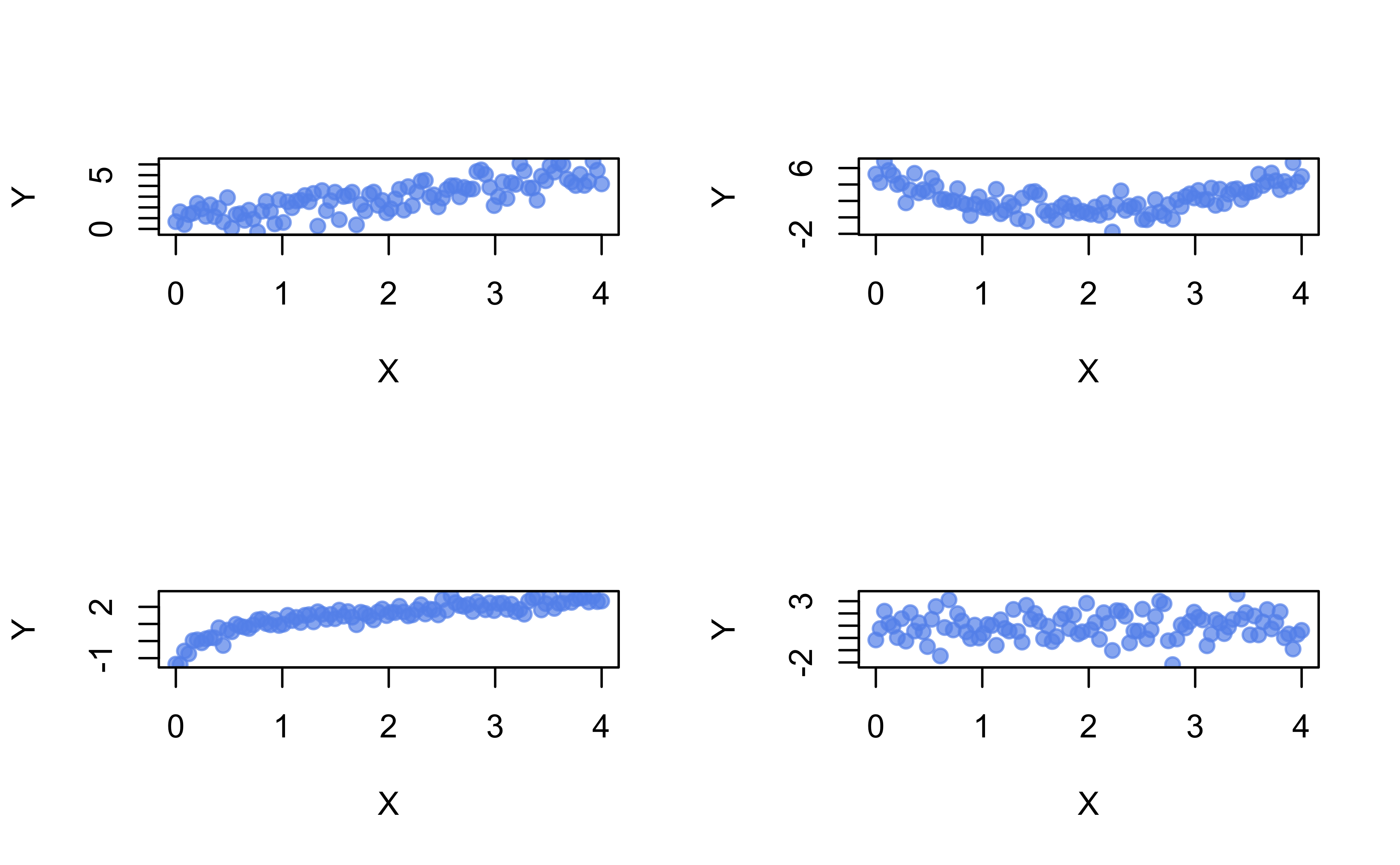
Are \(X\) and \(Y\) correlated?
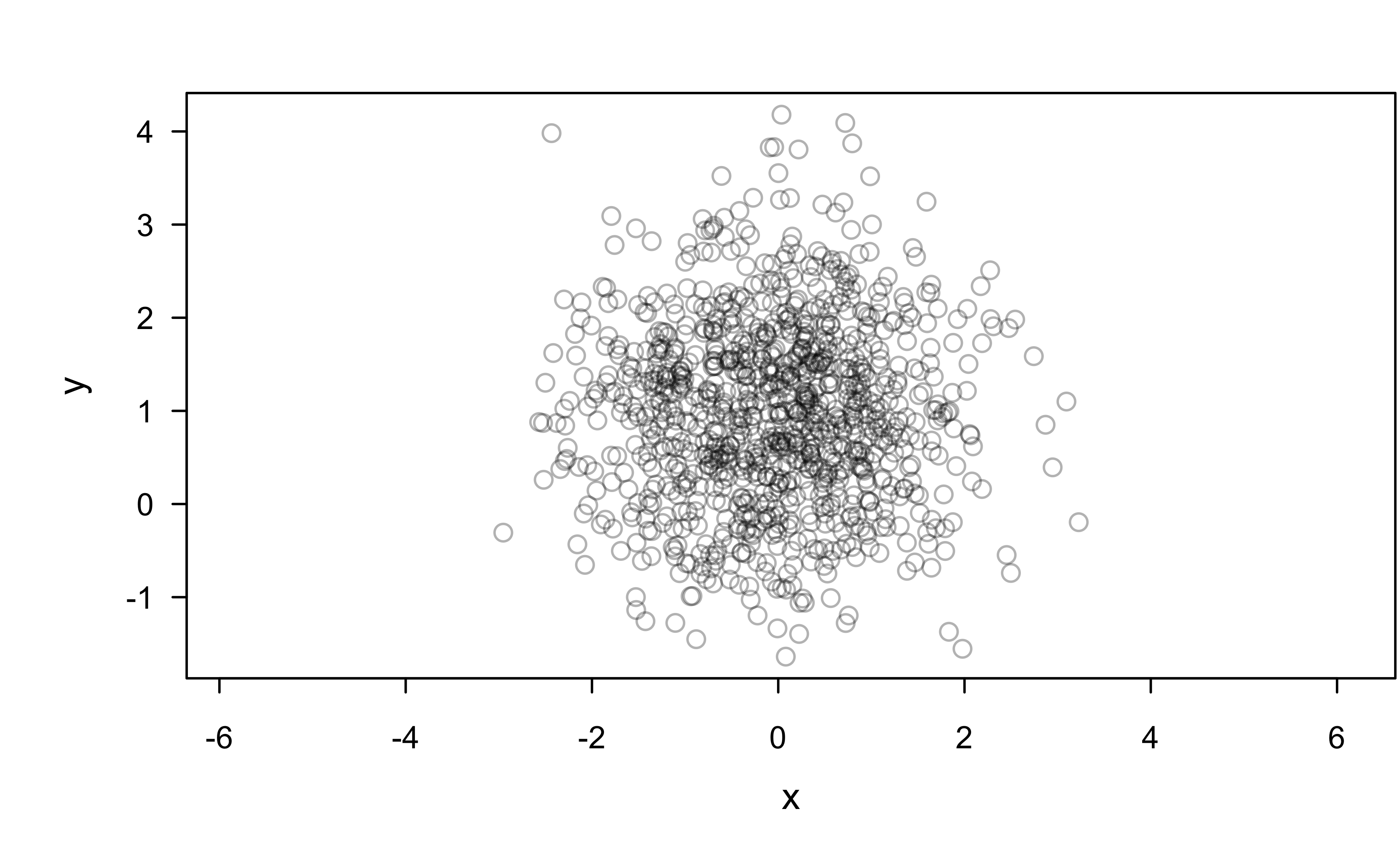
Are \(x\) and \(y\) correlated?
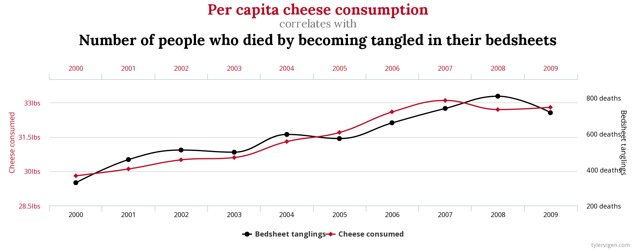
All models are wrong!
Also, see this talk by my old adviser, Thad Tarpey: “All Models are Right… most are useless.”
Statistical relationships
Show R code
library(ggplot2)

p1 <- ggplot(investr::crystal, aes(x = time, y = weight)) +
  geom_point() +
  labs(x = "Time (hours)",
       y = "Weight (grams)",
       title = "Crystal weight data")
p2 <- ggplot(investr::arsenic, aes(x = actual, y = measured)) +
  geom_point() +
  labs(x = "True amount of arsenic",
       y = "Measured amount of arsenic",
       title = "Arsenic concentration data")
gridExtra::grid.arrange(p1, p2, nrow = 1)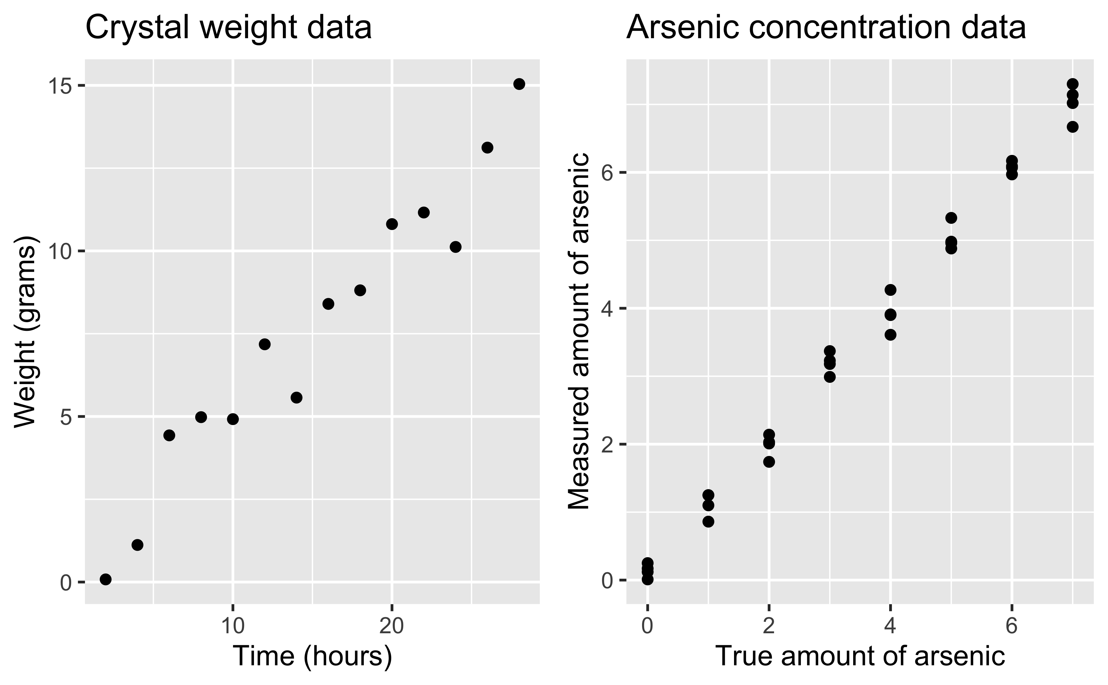
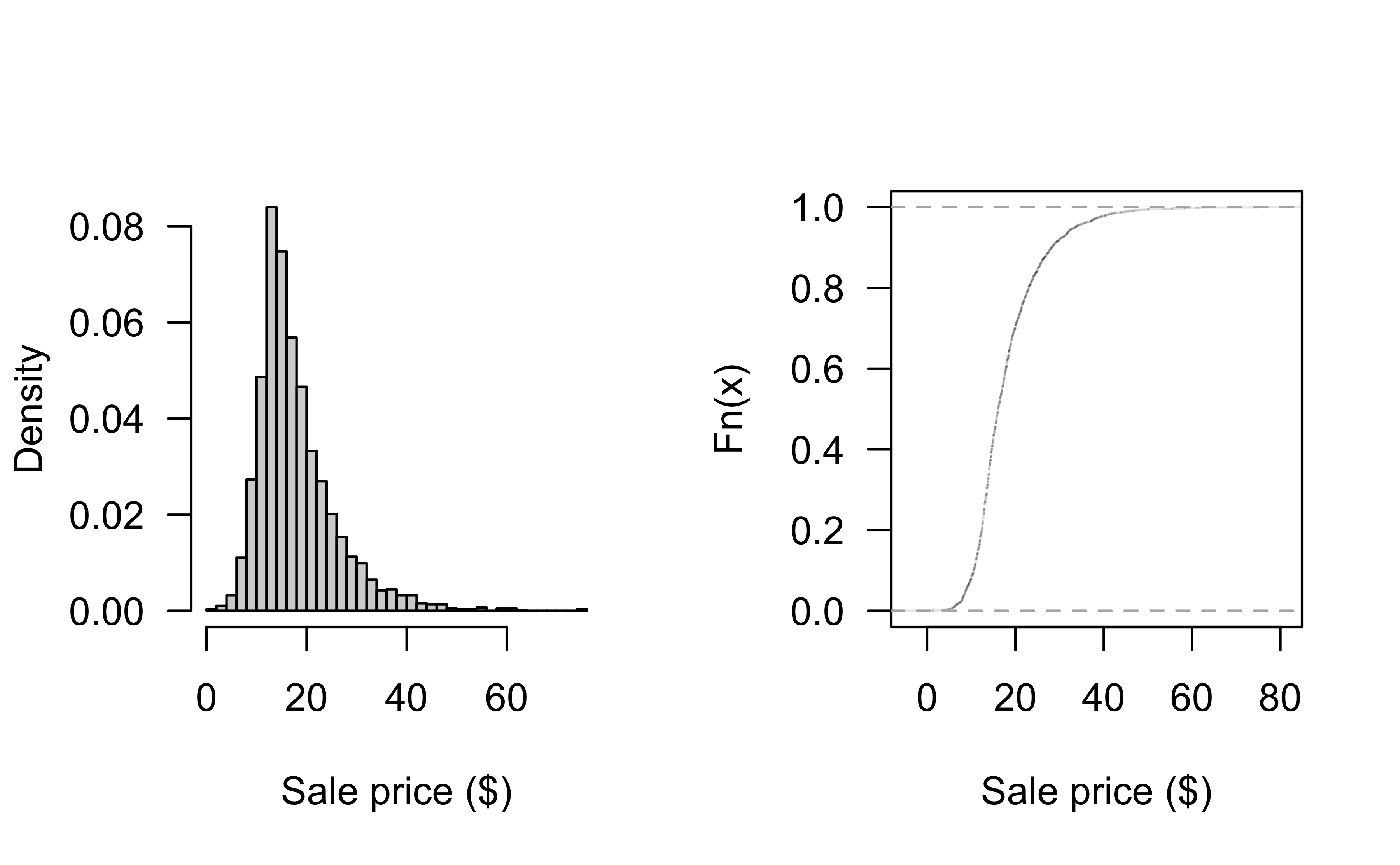
Distribution of Sale_Price
Can look at historgram and empirical CDF:
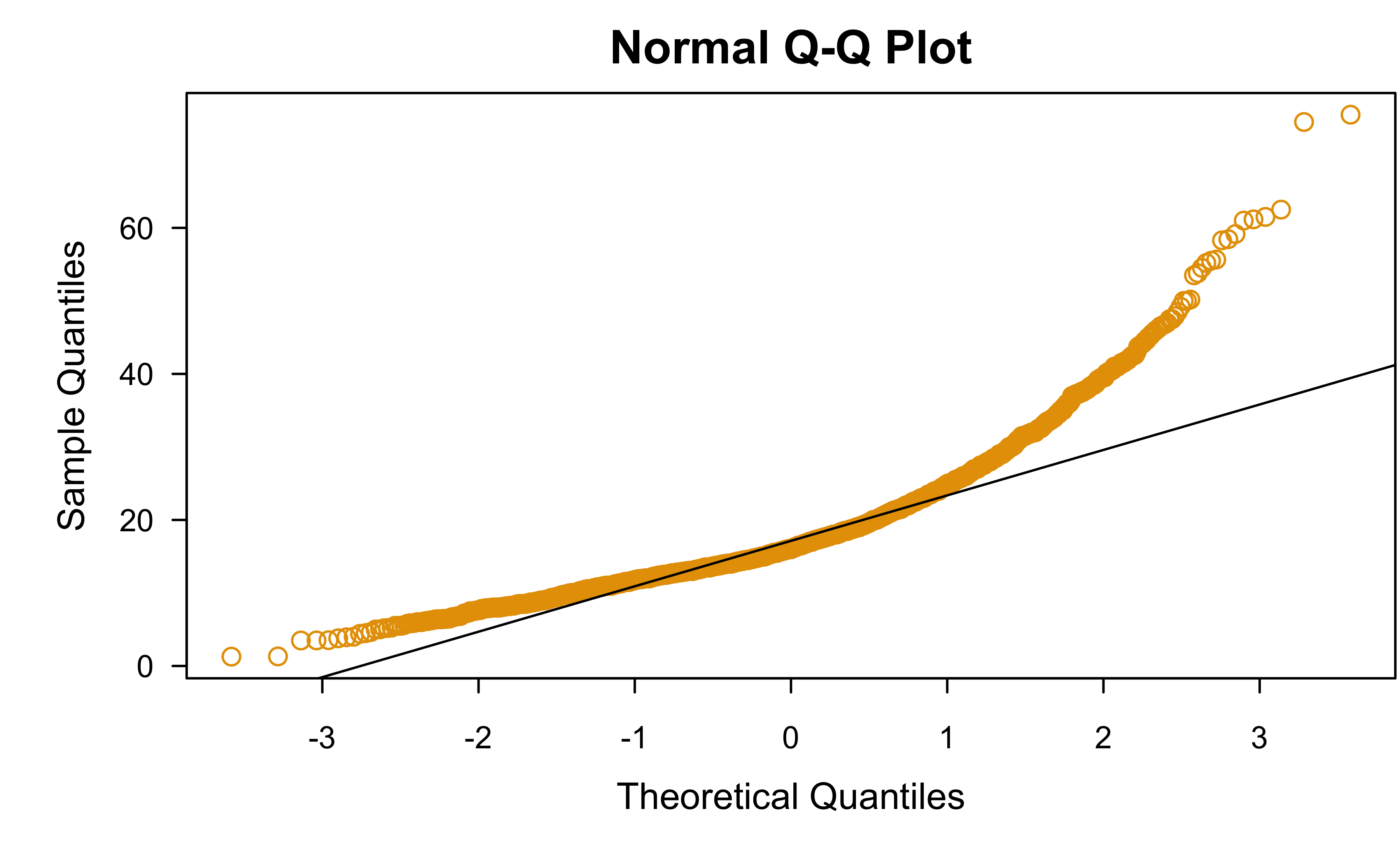
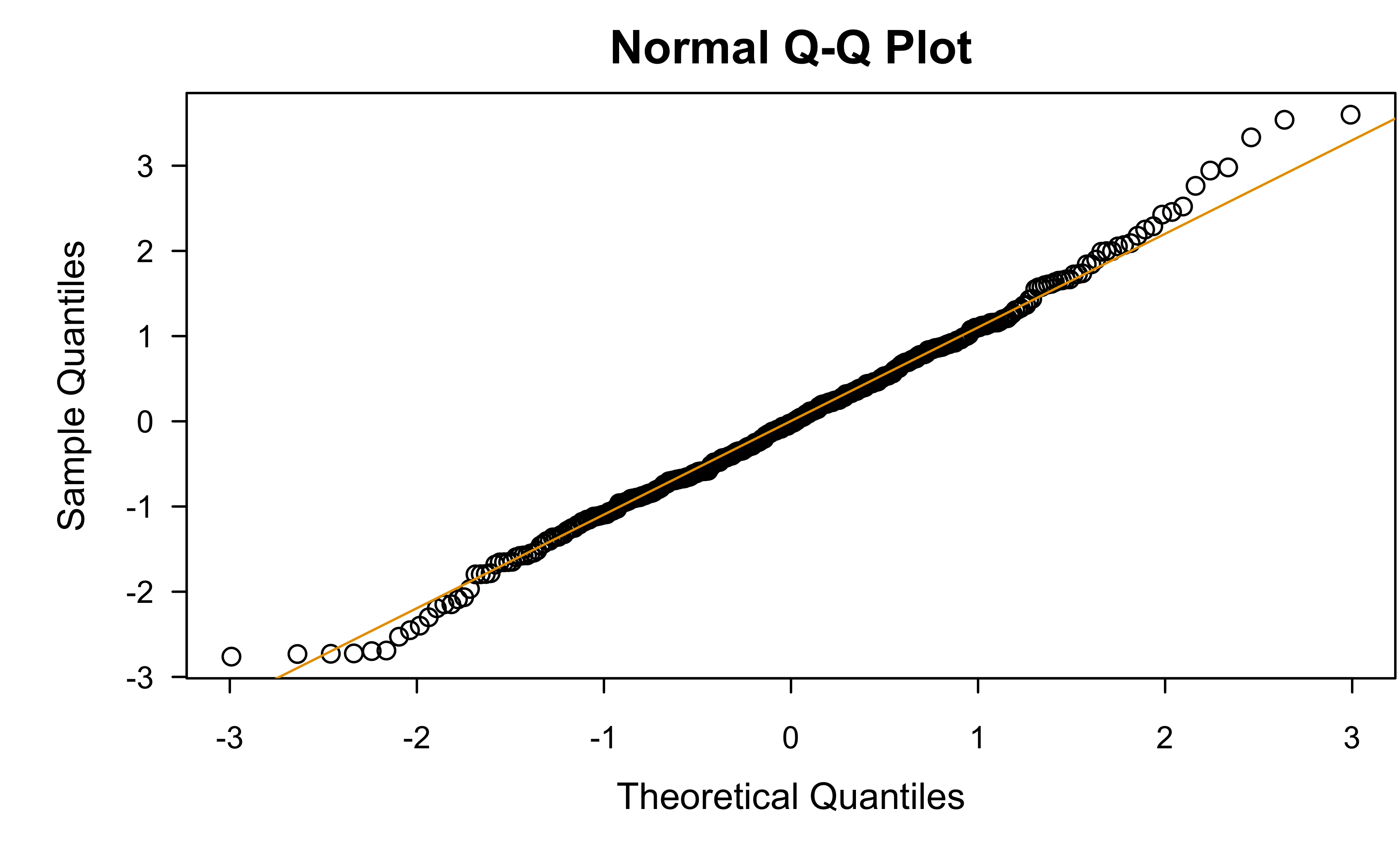
Normal QQ plot
Normal quantile-quantile (Q-Q) plot* can be used to asses the “normalityness” of a set of observations
Q-Q plots can, in general, be used to compare data with any distribution!
Normality tests 🤮
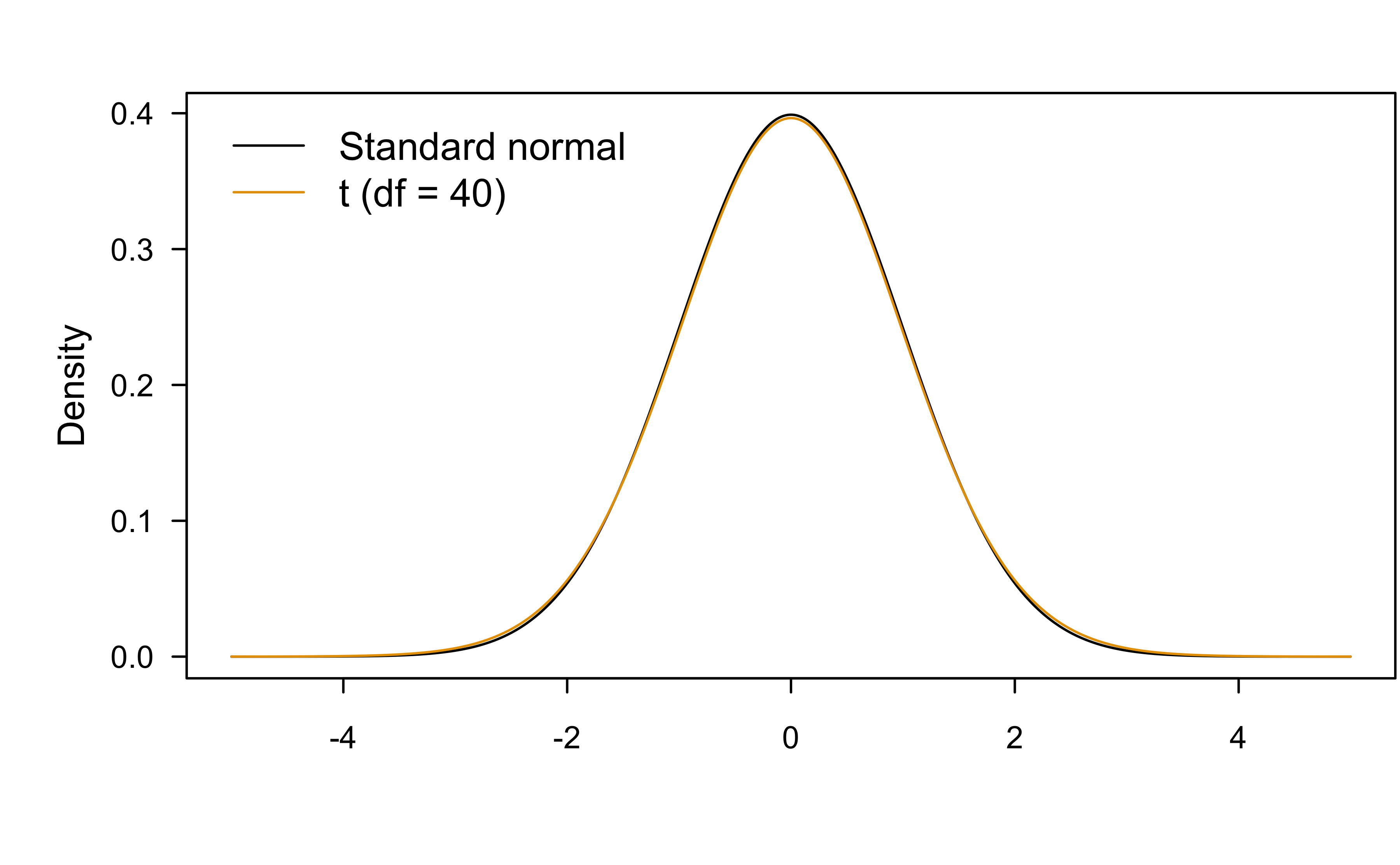
Are these two distributions significantly different?
Are these two distributions practically different?
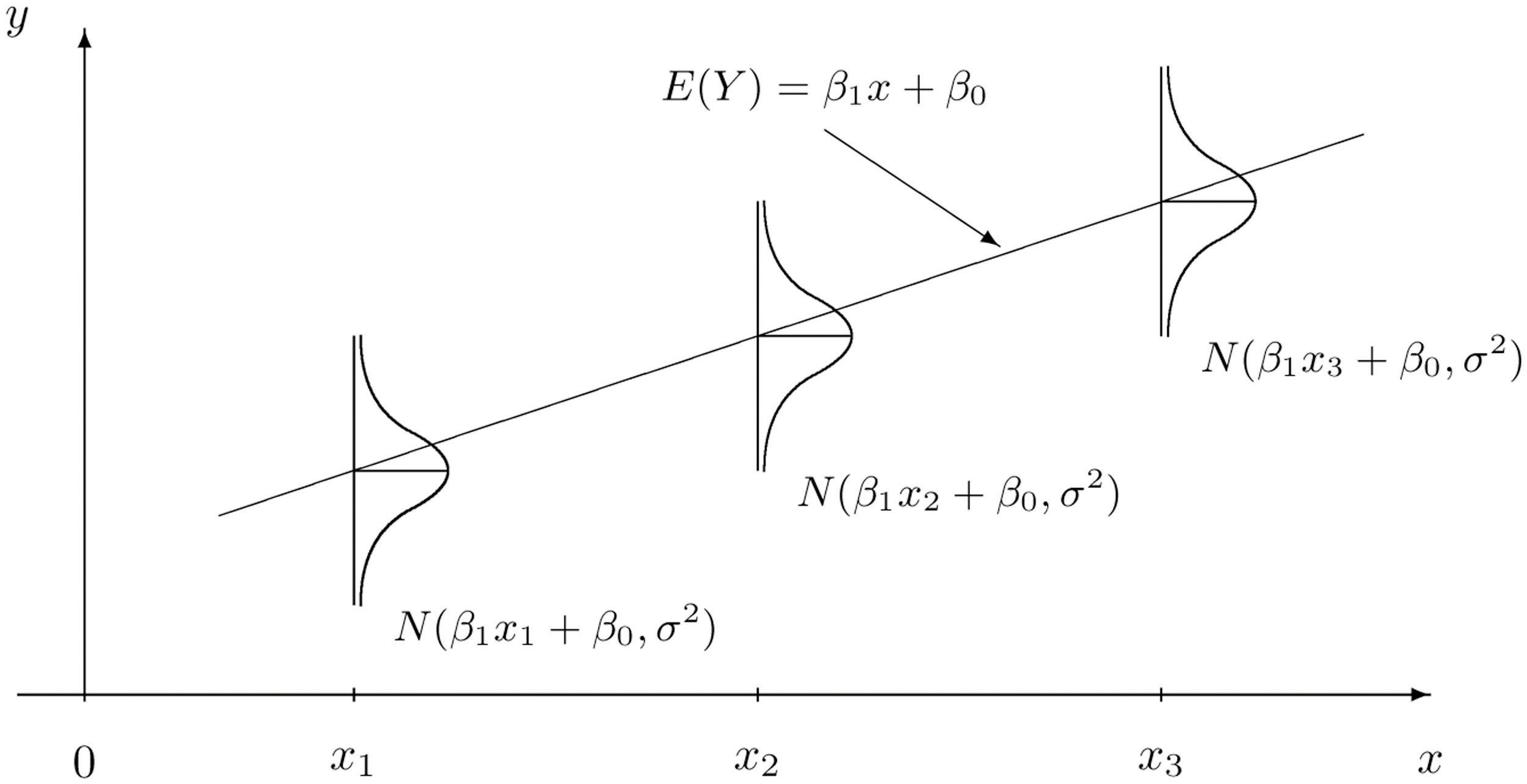
The idea behind SLR
Arsenic experiment example
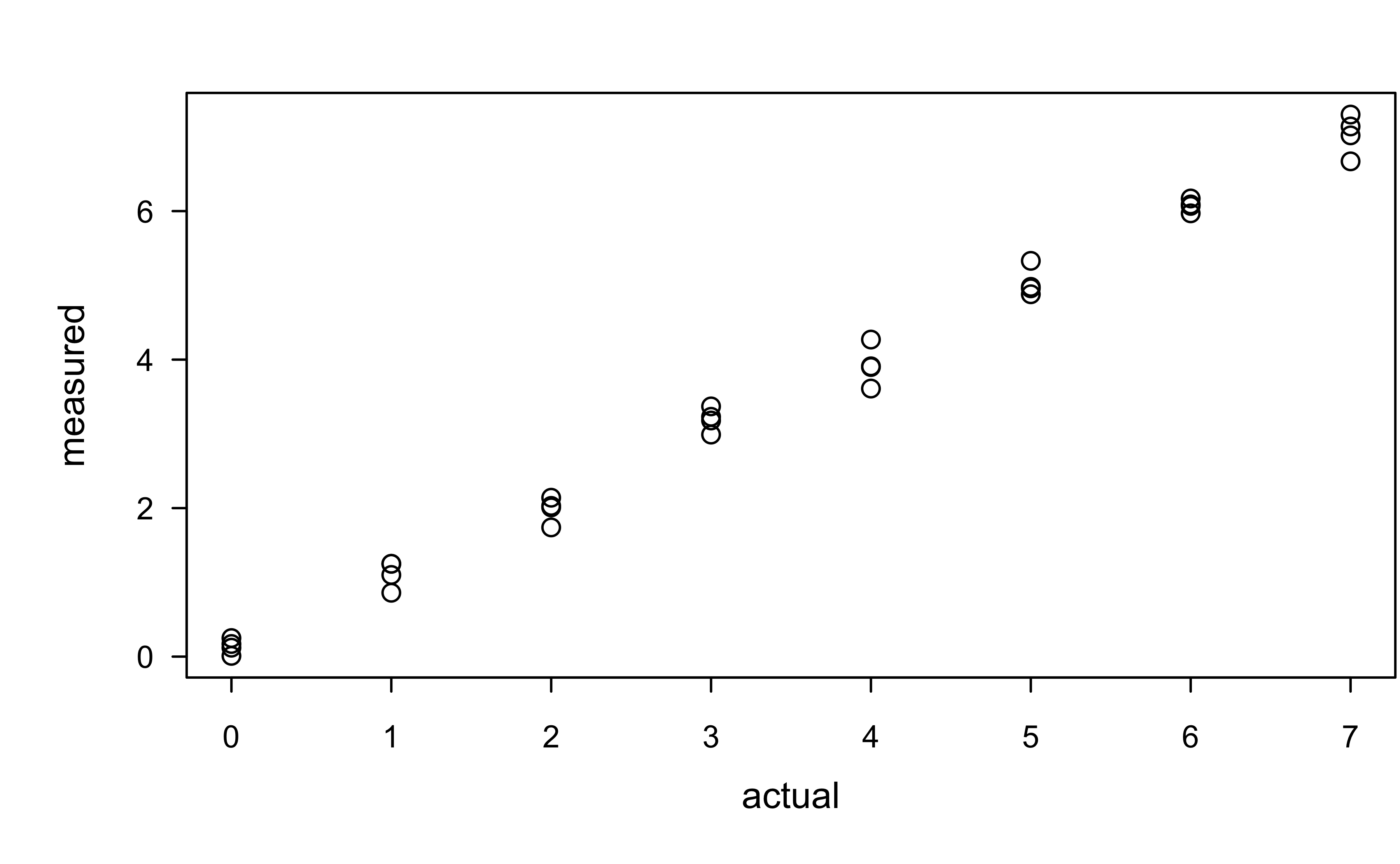
Is linear regression reasonable here?
Is linear regression reasonable here?
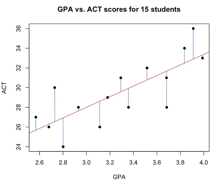
Concept of LS estimation
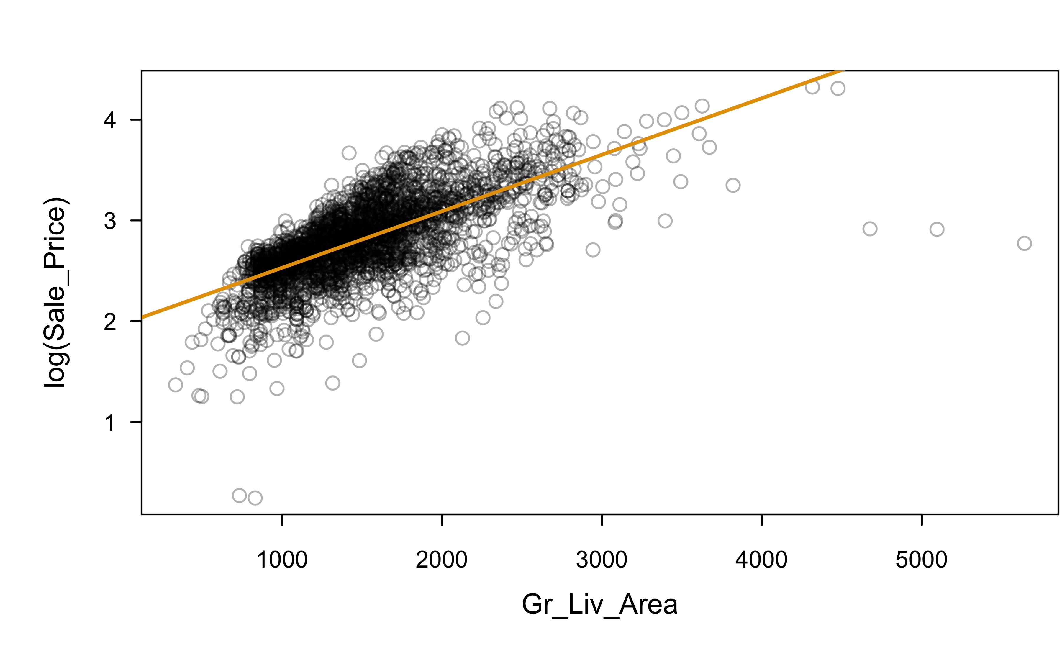
Sale_Price and Gr_Liv_Area
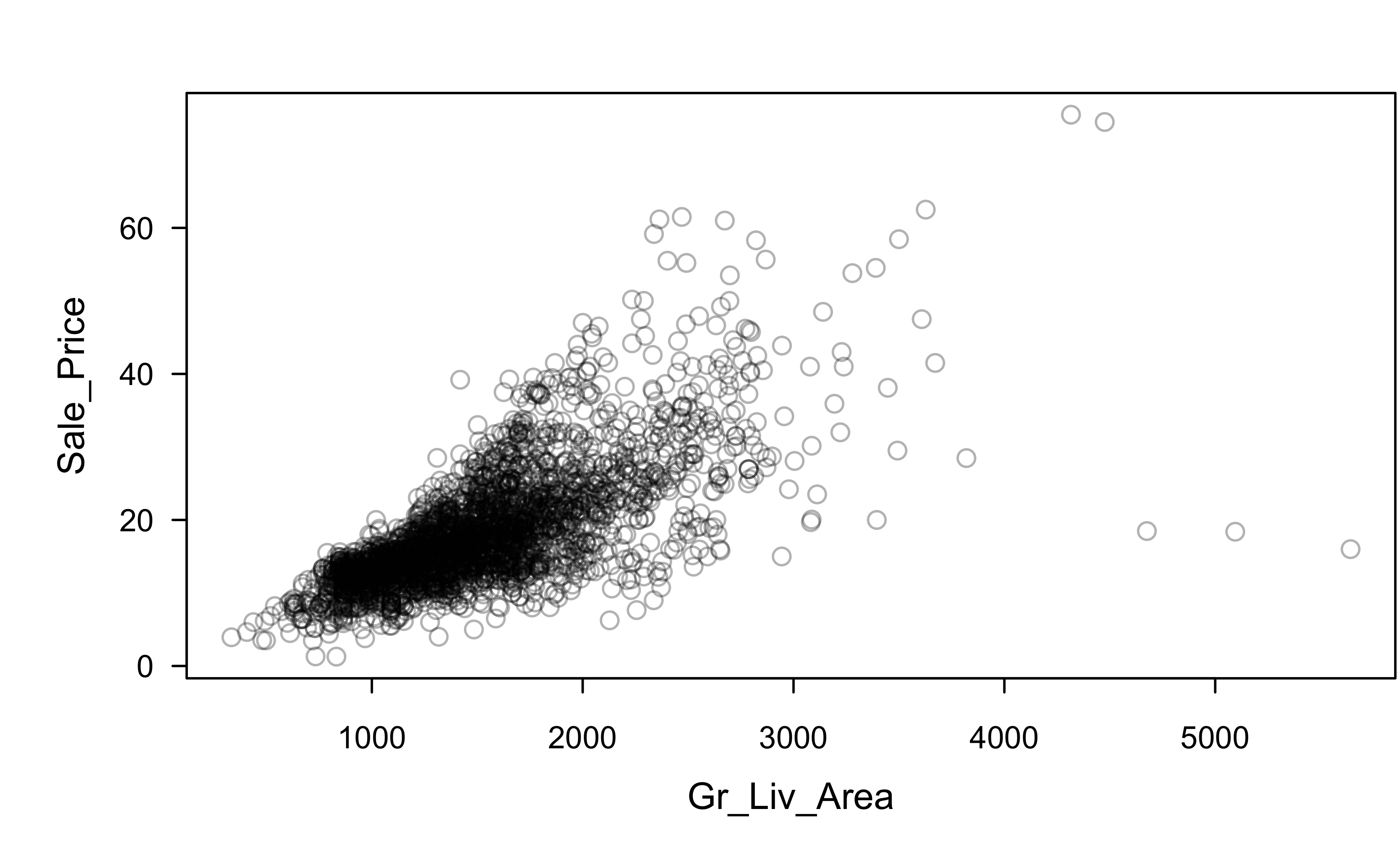
Is this a good fit?
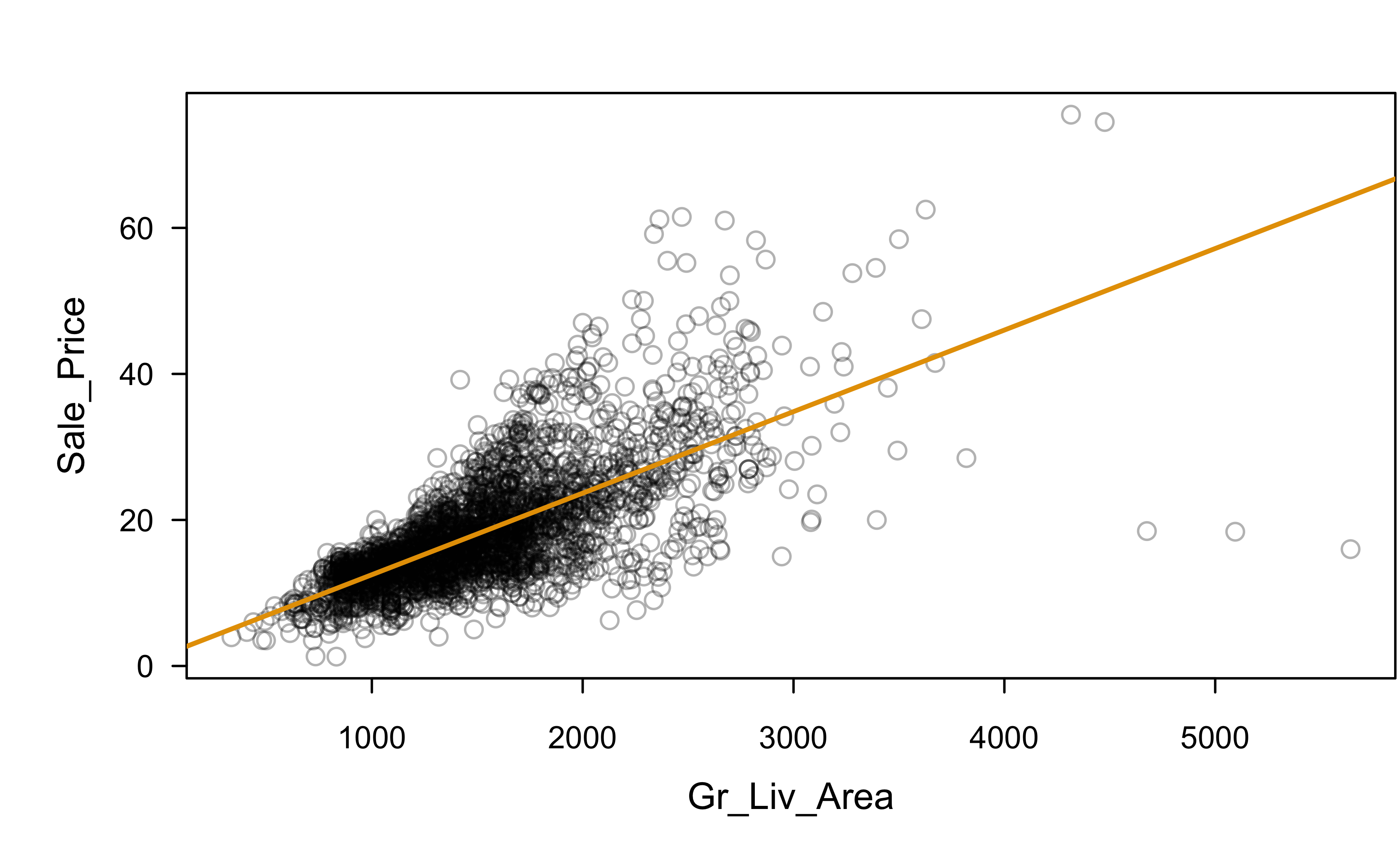
Which assumptions seem violated to some degree?
Sale_Price ~ Gr_Liv_Area
Residual analysis:
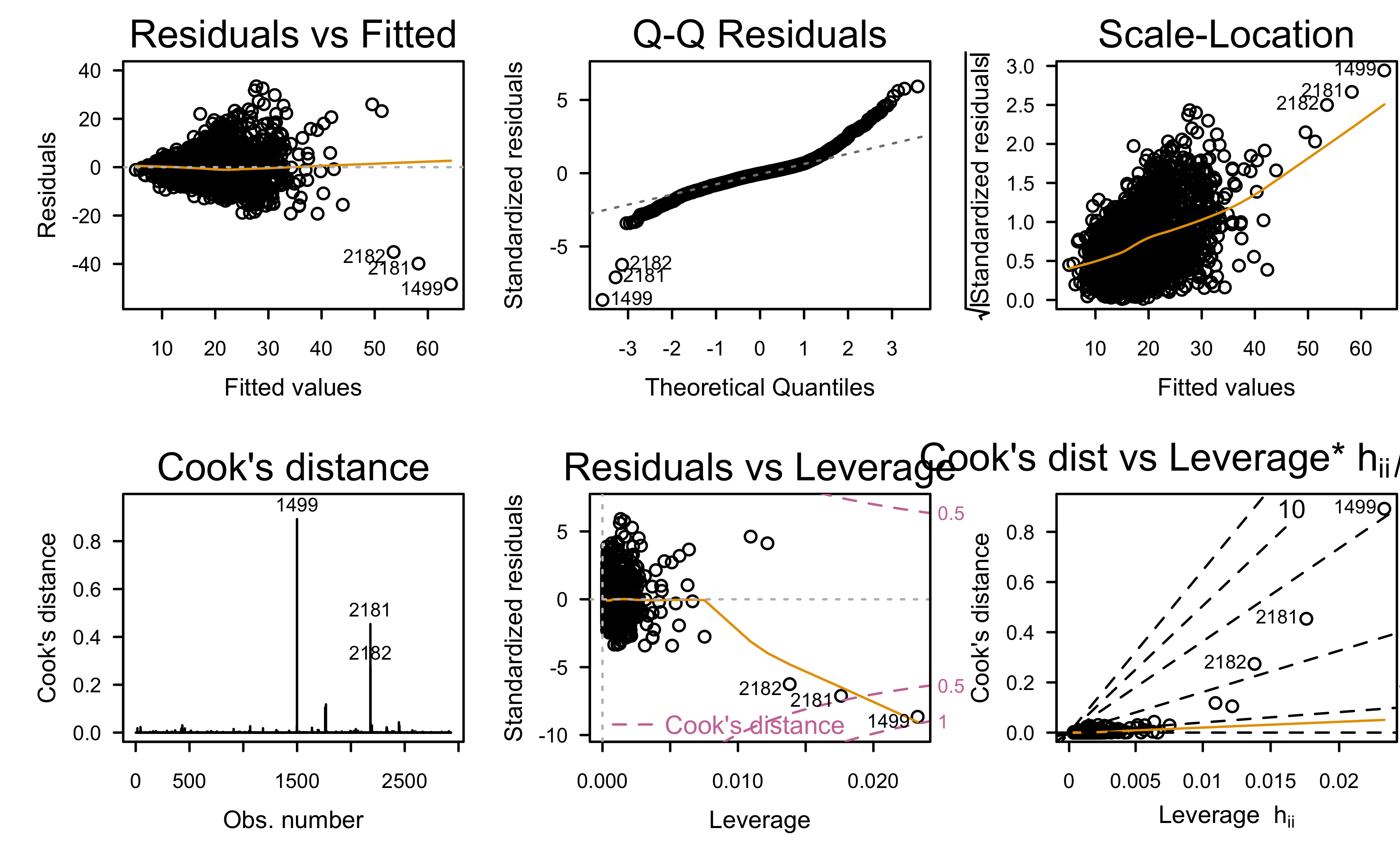
What assumptions appear to be in violation?
Let’s try a log transformation
log(Sale_Price) ~ Gr_Liv_Area
Residual analysis:
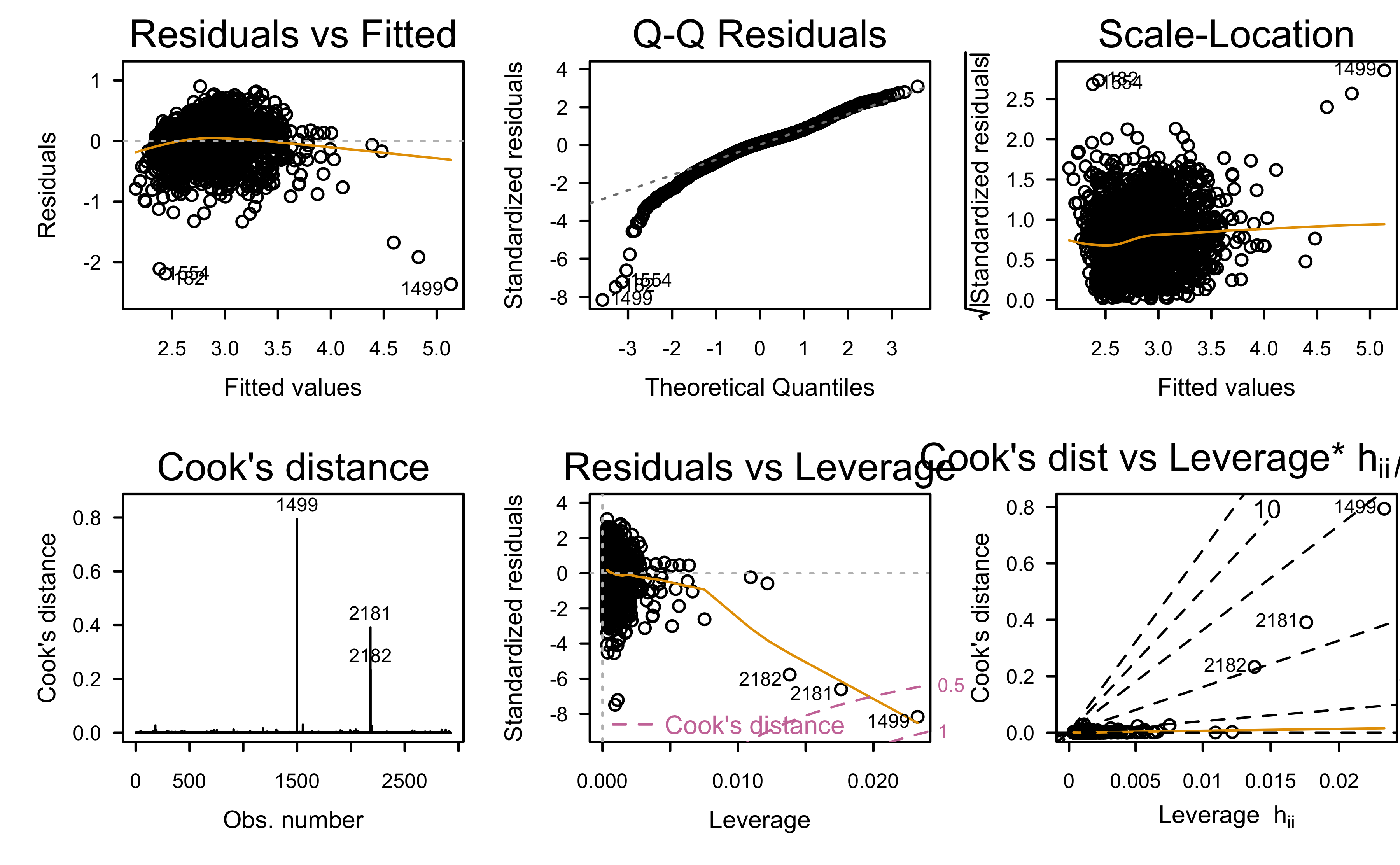
Any better?
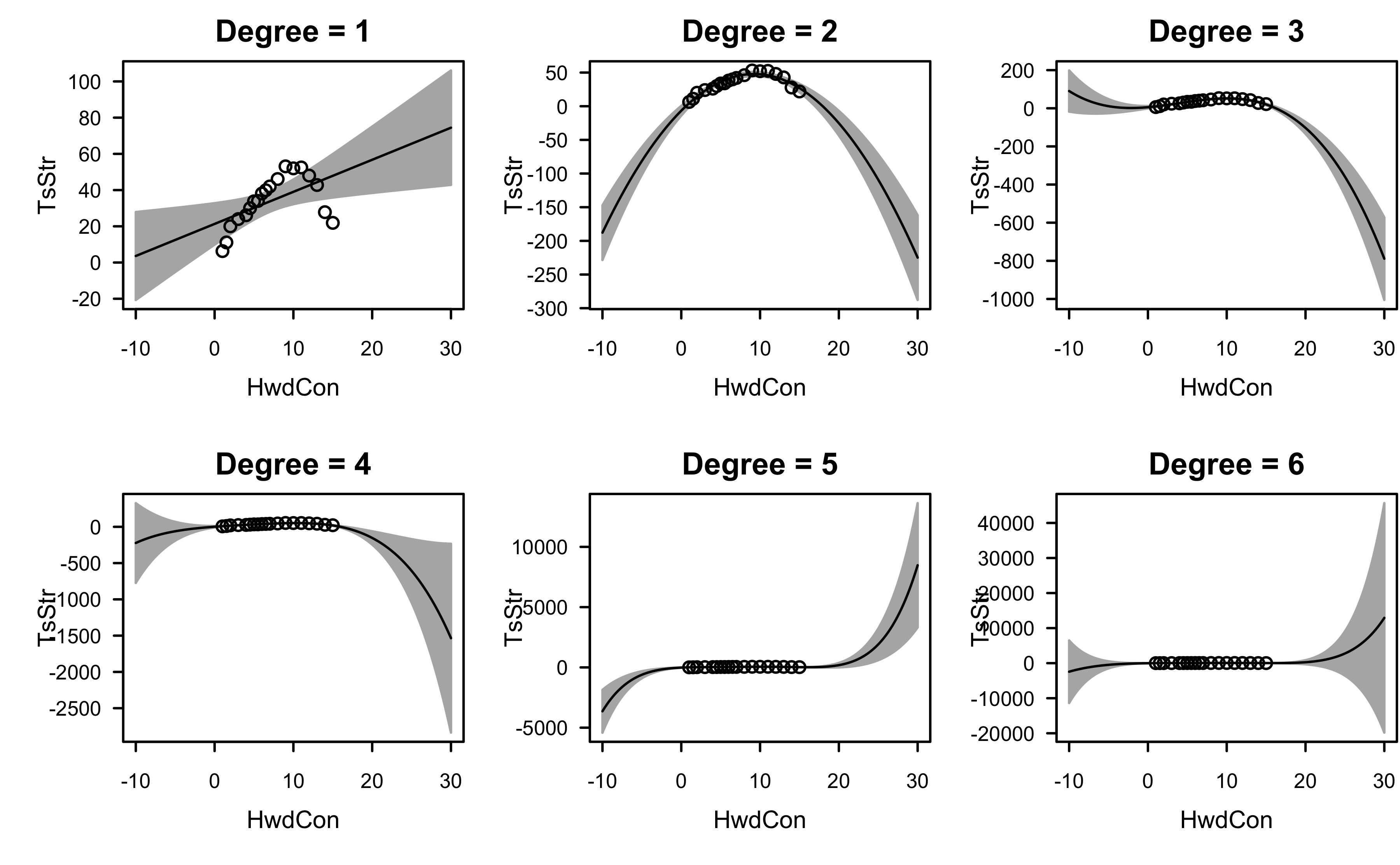
Example: paper strength data
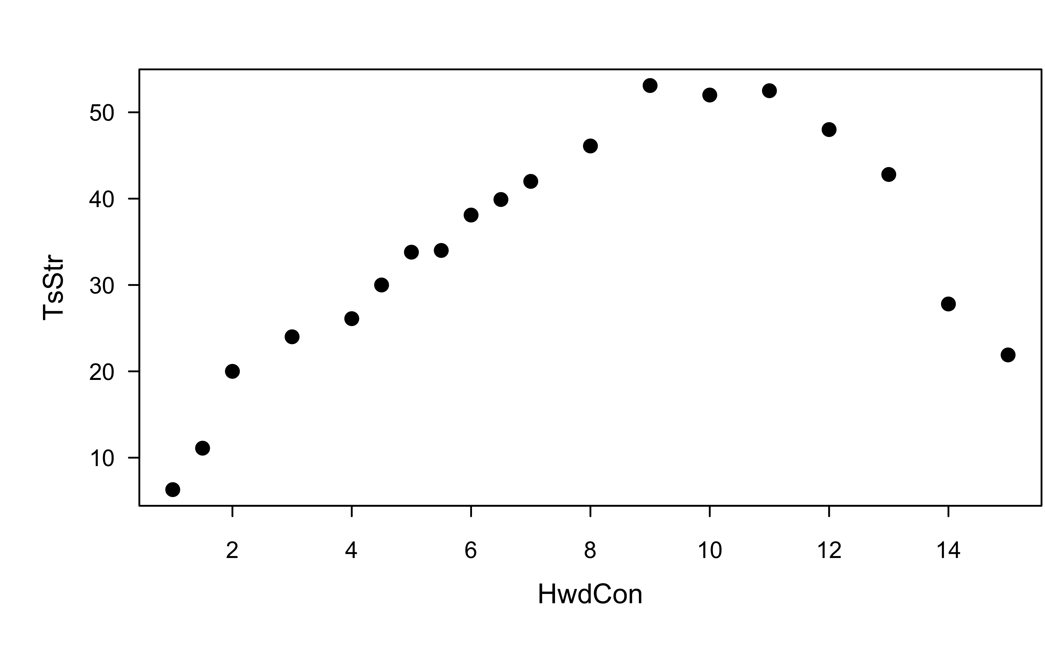
Example: paper strength data
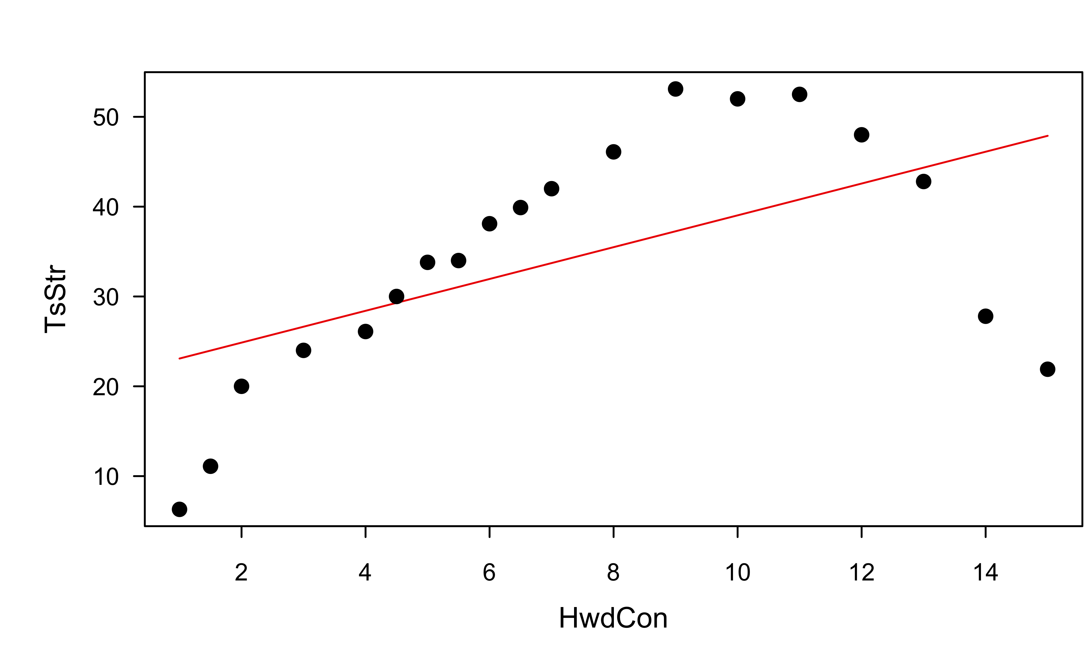
Example: paper strength data
Show R code
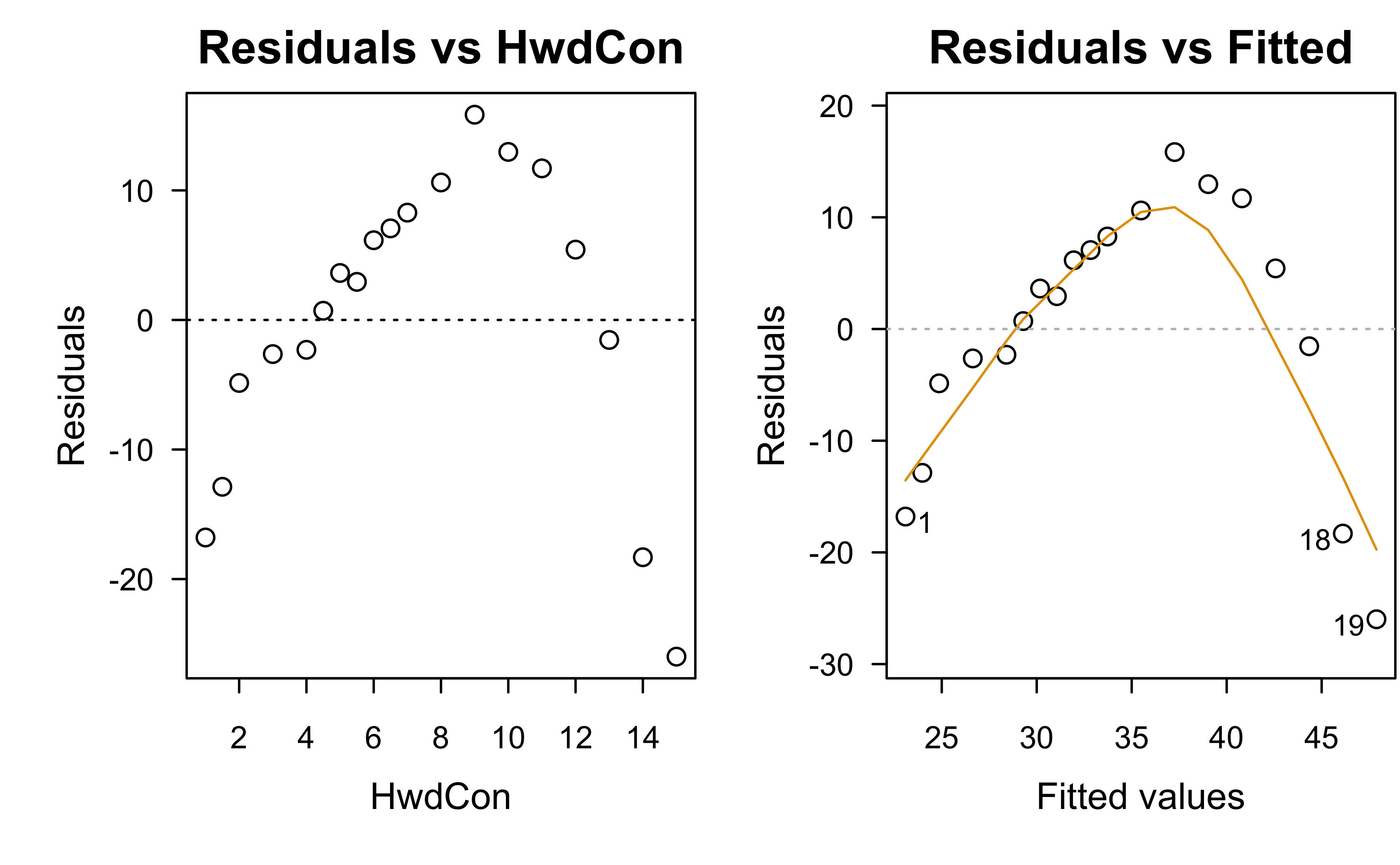
Example: paper strength data
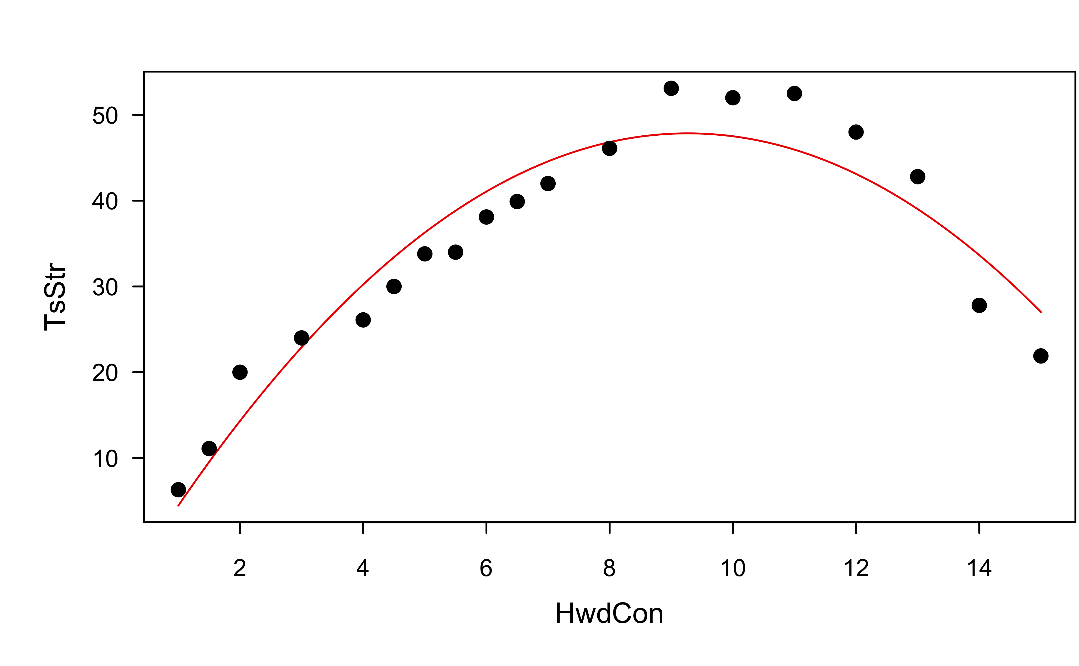
Example: paper strength data
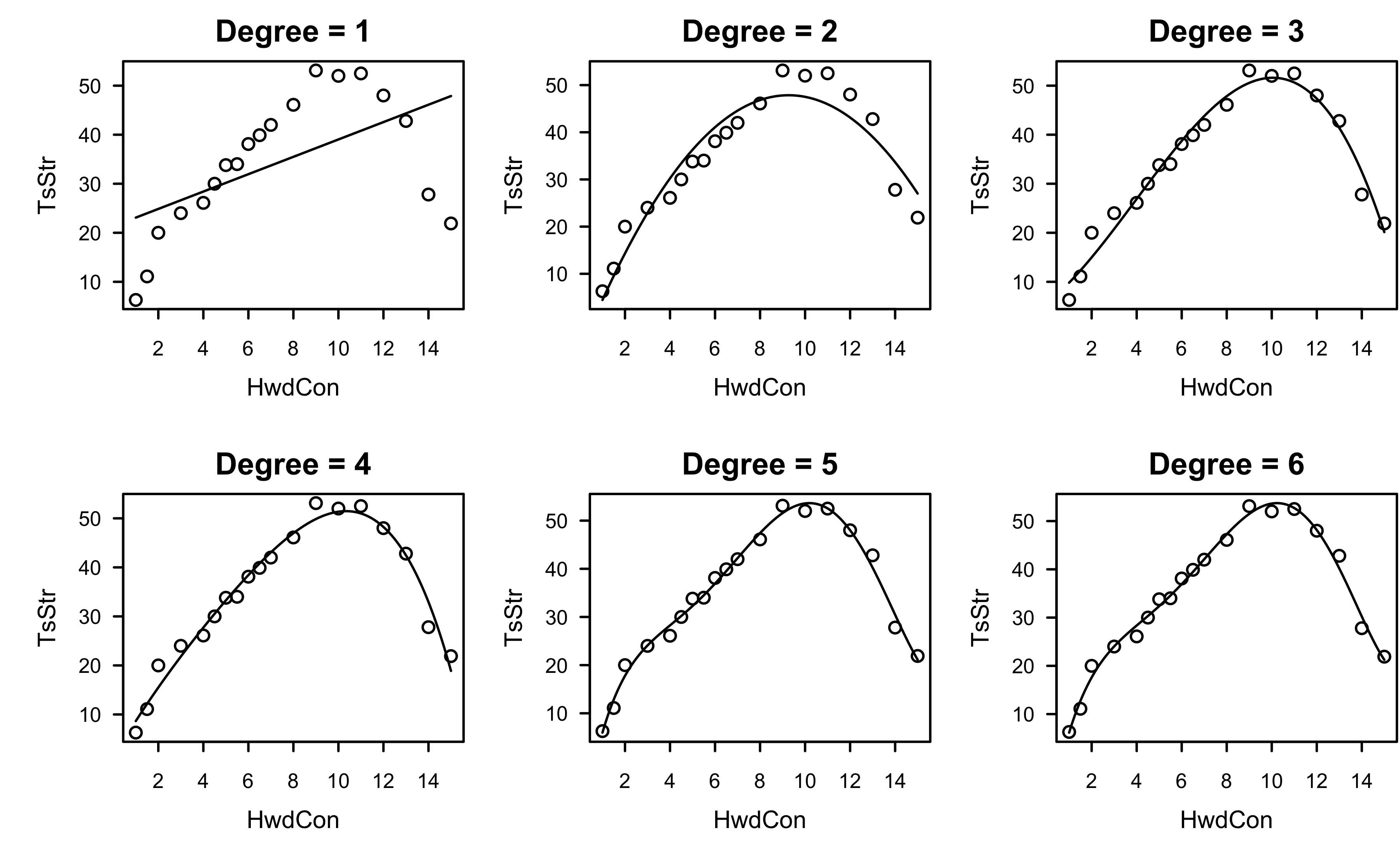
Example: paper strength data
Categorical variables
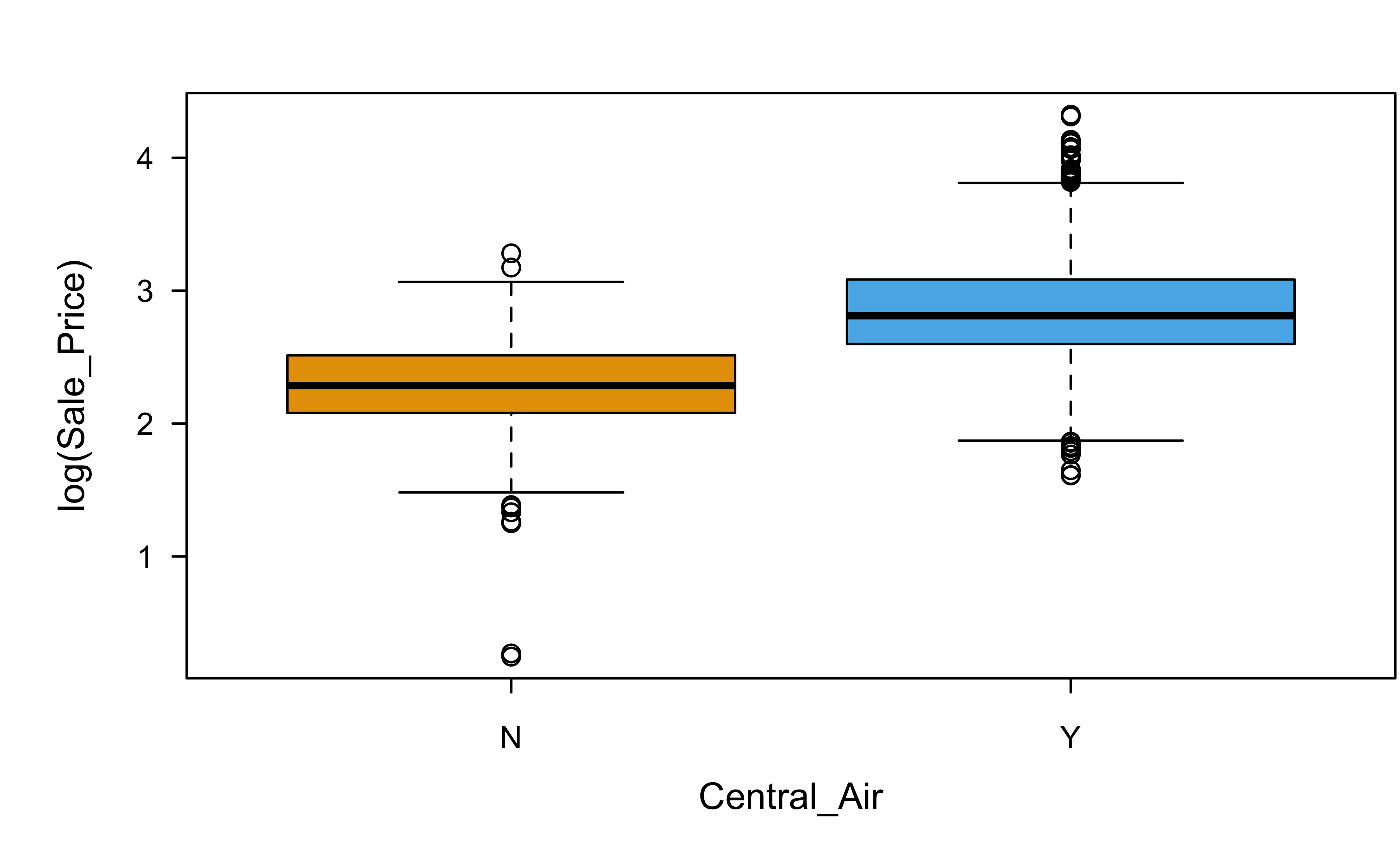
Categorical variables
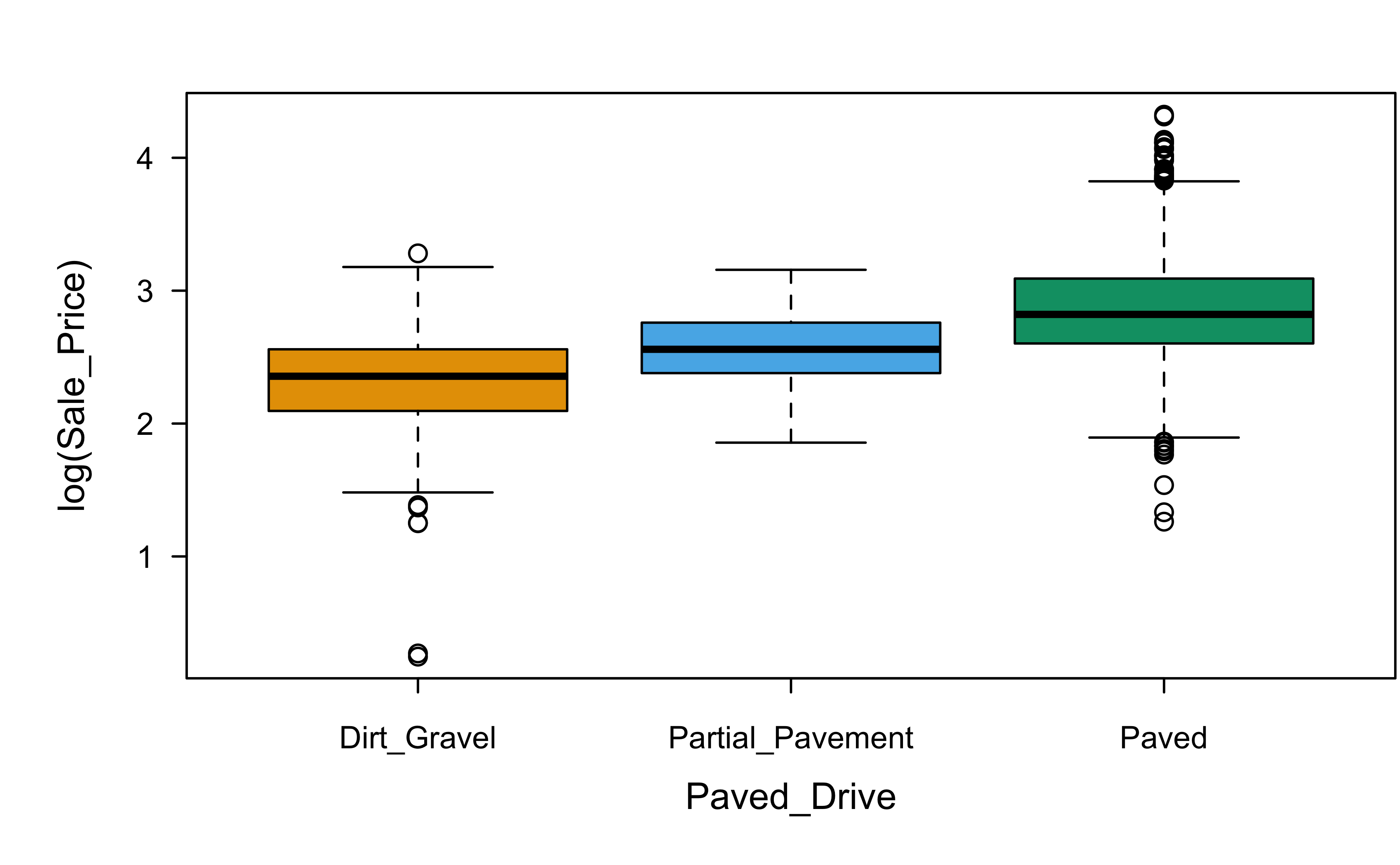
If one of these homes downgraded from a paved driveway to a gravel driveway, would that cause the sale price to decrease? (Think very carefully here!)
Data splitting: \(k\)-fold cross-validation
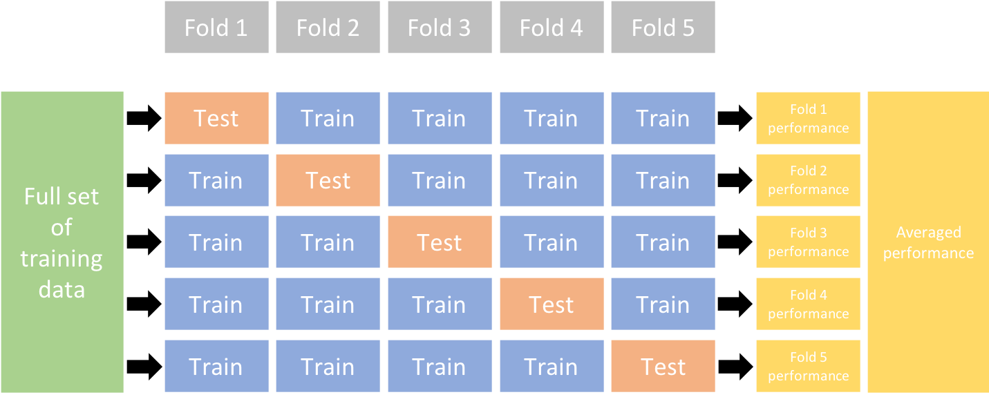
The PRESS statistic in linear regression is a special case (\(k = n\)) we get for free!