Linear Regression
A Brief Review
About me


Statistical relationships
Show R code
# Simulate data from different SLR models
set.seed(101)  # for reproducibility
x <- seq(from = 0, to = 4, length = 100)
y <- cbind(
  1 + x + rnorm(length(x)),  # linear
  1 + (x - 2)^2 + rnorm(length(x)),  # quadratic
  1 + log(x + 0.1) + rnorm(length(x), sd = 0.3),  # logarithmic
  1 + rnorm(length(x))  # no association
)

# Scatterplot of X vs. each Y in a 2-by-2 grid
par(mfrow = c(2, 2))
for (i in 1:4) {
  plot(x, y[, i], col = adjustcolor("cornflowerblue", alpha.f = 0.7),
       pch = 19, xlab = "X", ylab = "Y")
}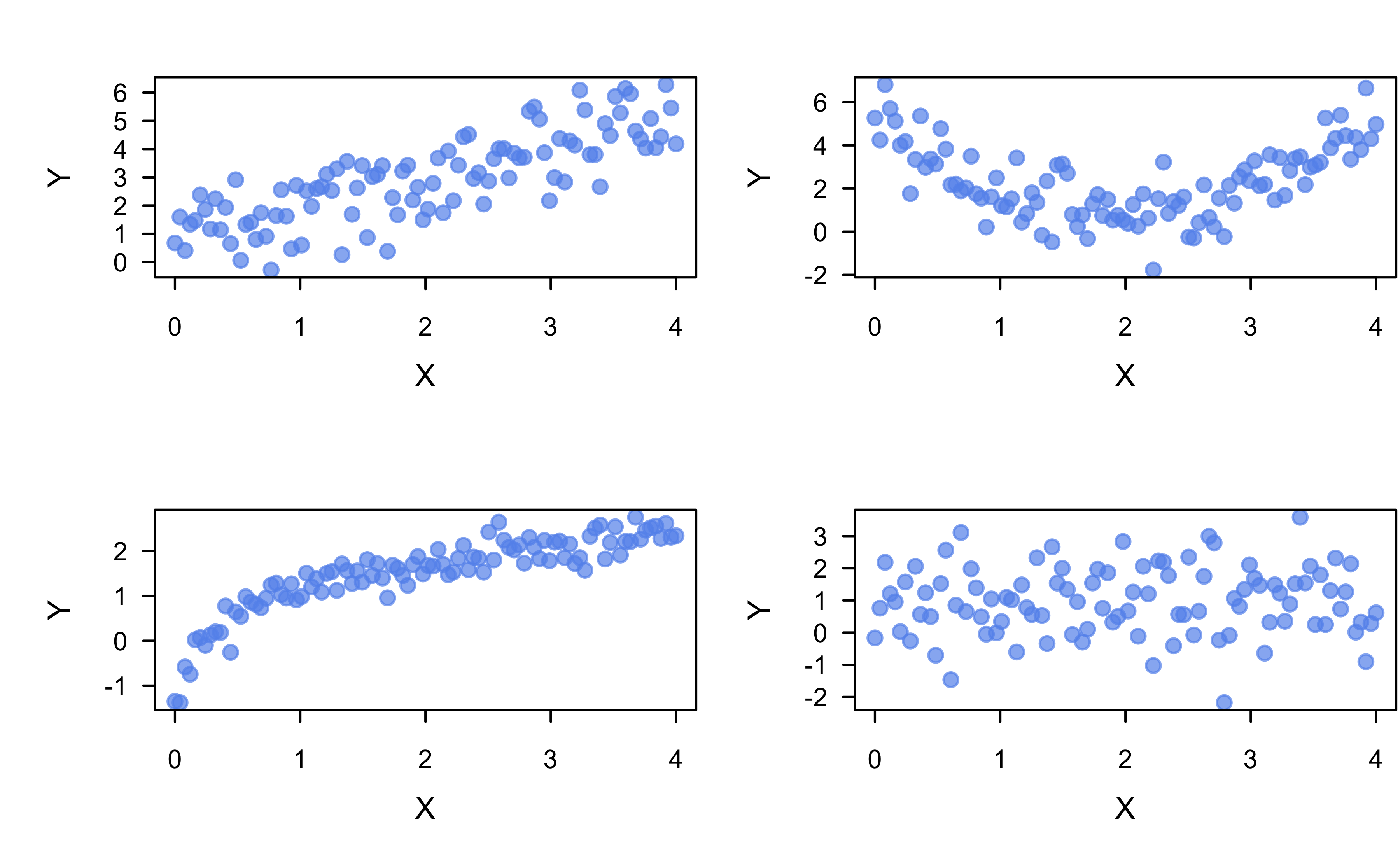
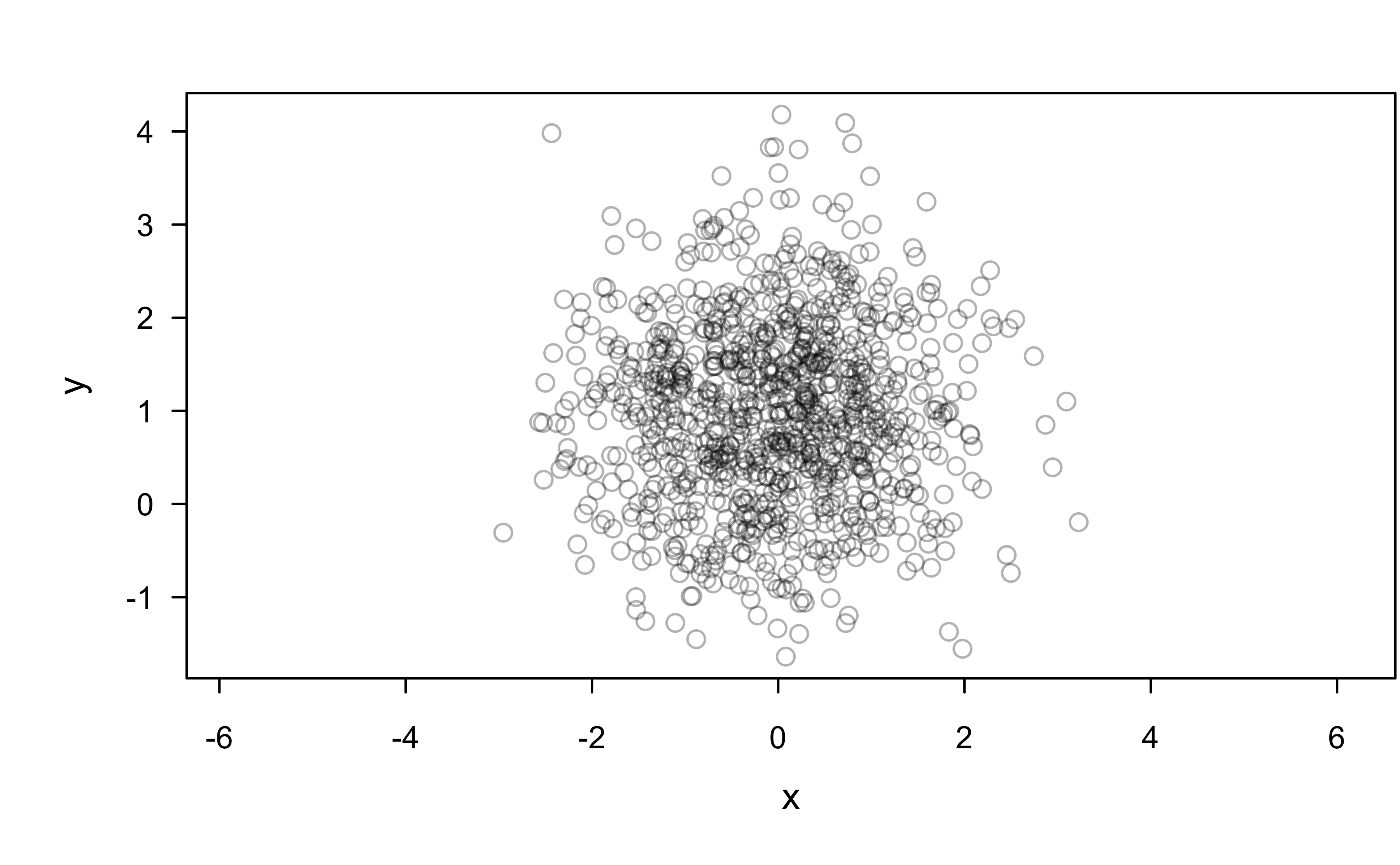
Are \(x\) and \(y\) correlated?
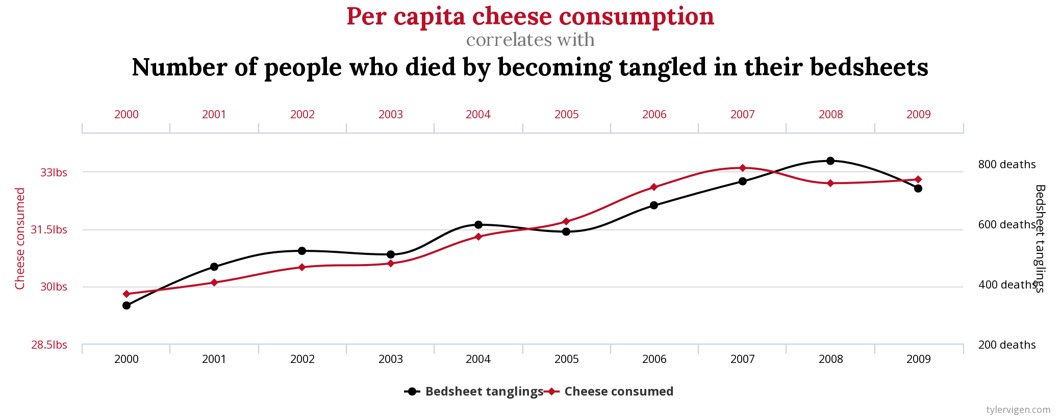
All models are wrong!

Also, see this talk by my old adviser, Thad Tarpey: “All Models are Right… most are useless.”
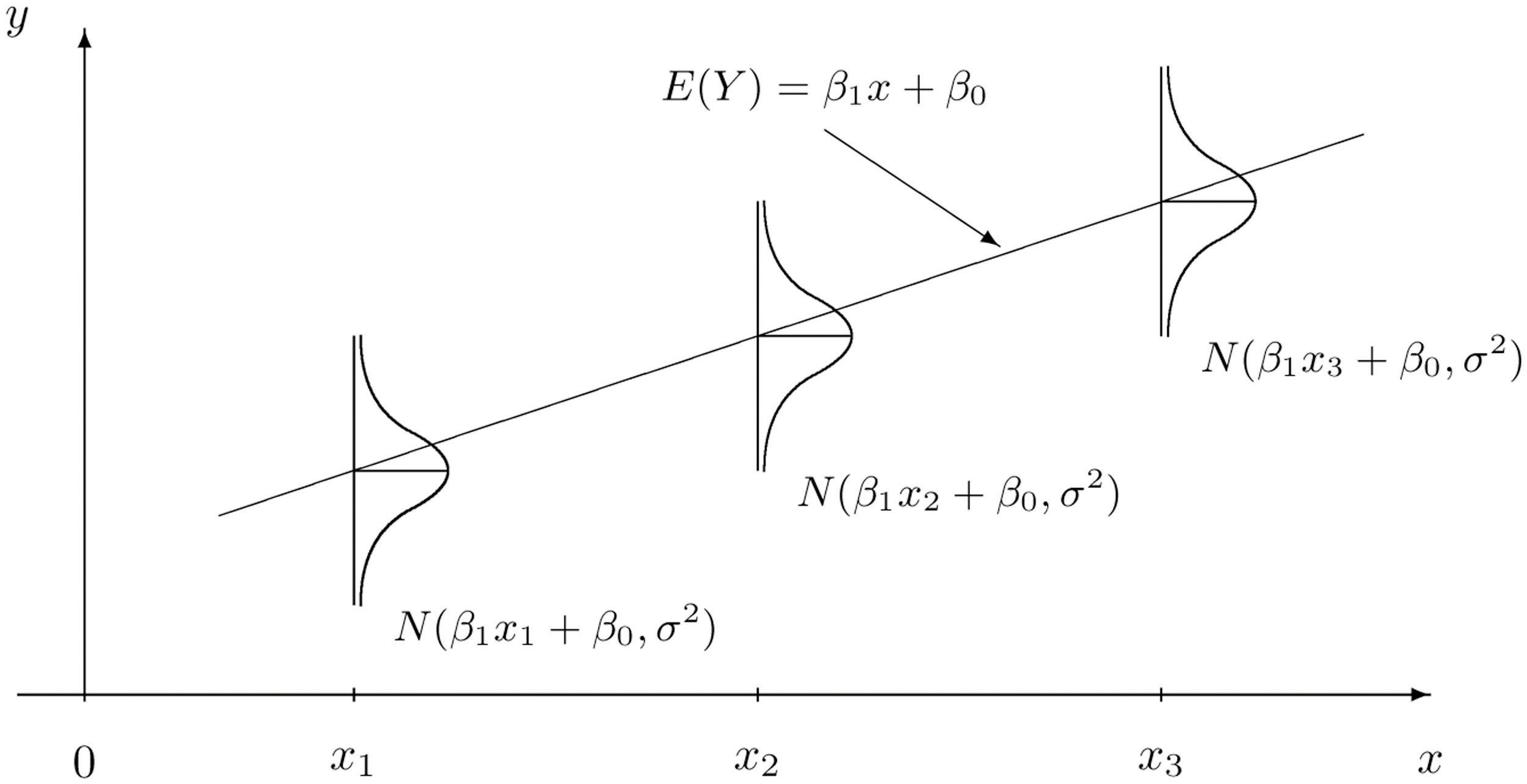
The idea behind SLR
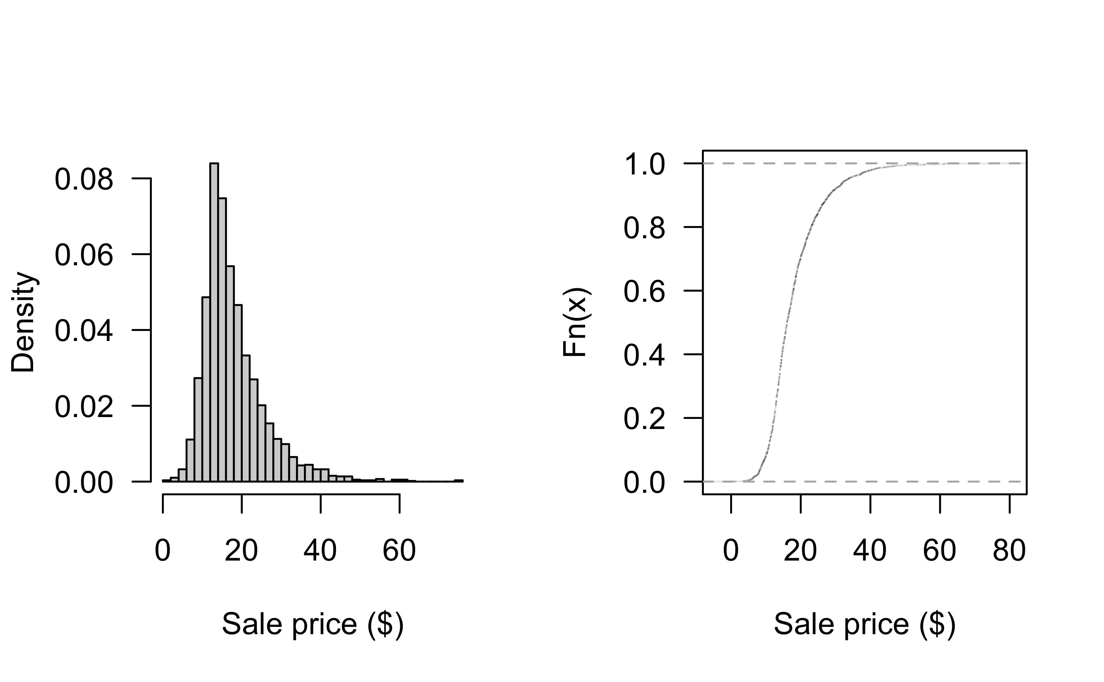
Distribution of Sale_Price
Can look at historgram and empirical CDF:
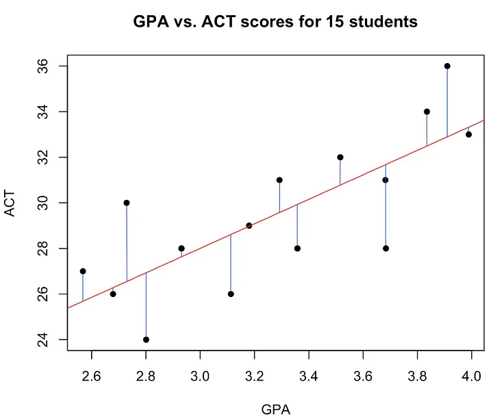
Concept of LS estimation
Sale_Price and Gr_Liv_Area
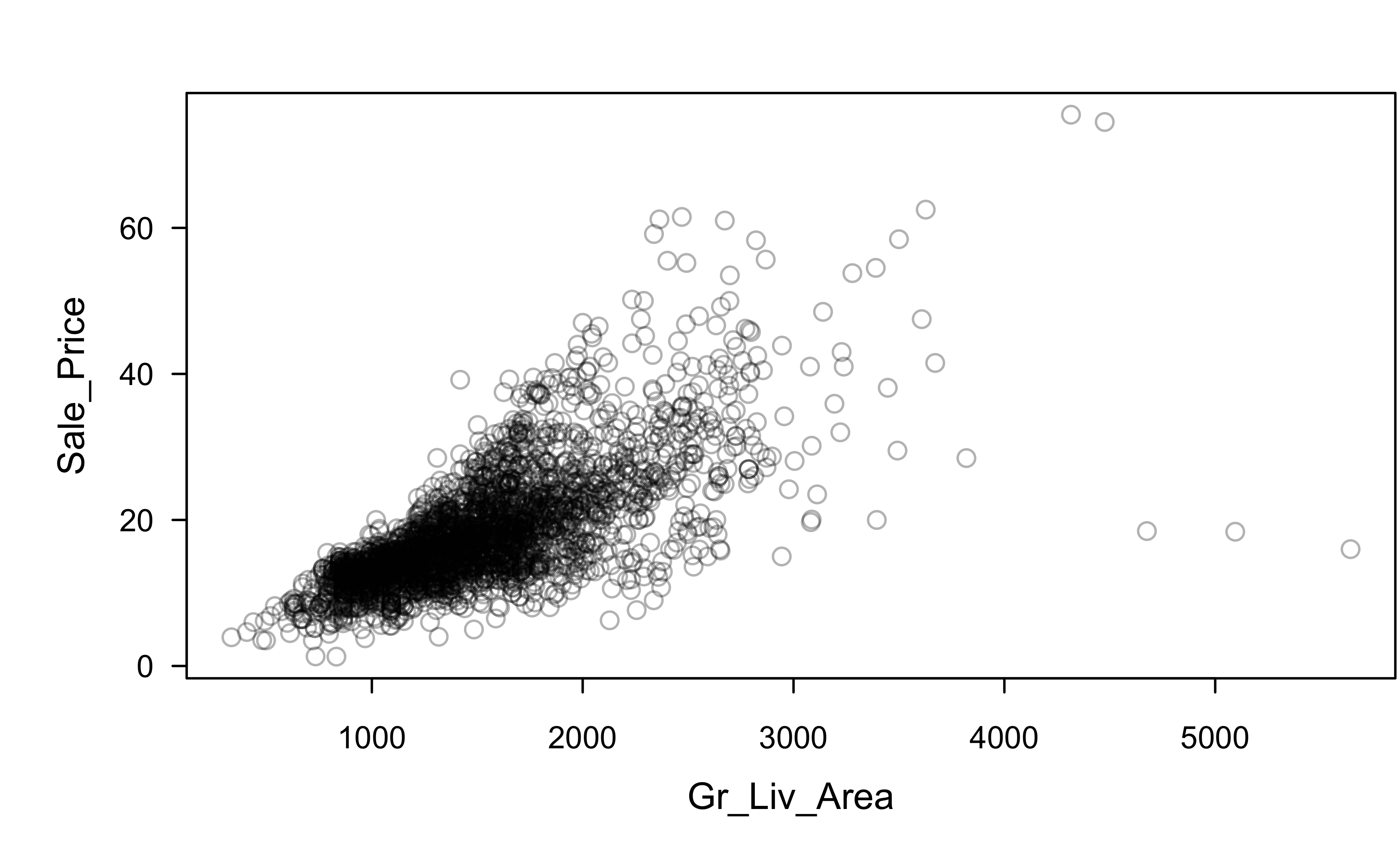
Is this a good fit?
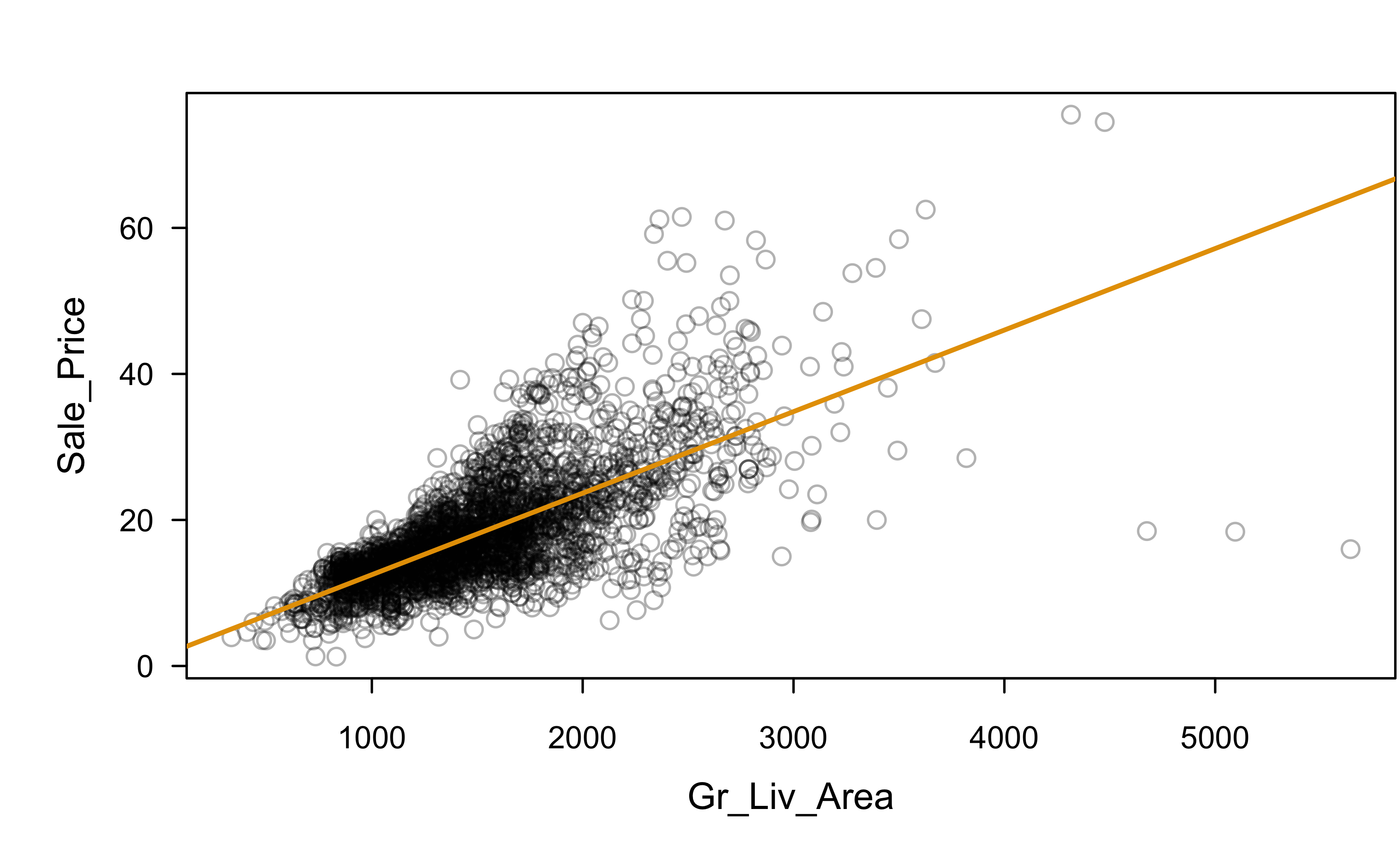
Which assumptions seem violated to some degree?
Sale_Price ~ Gr_Liv_Area
Residual analysis:
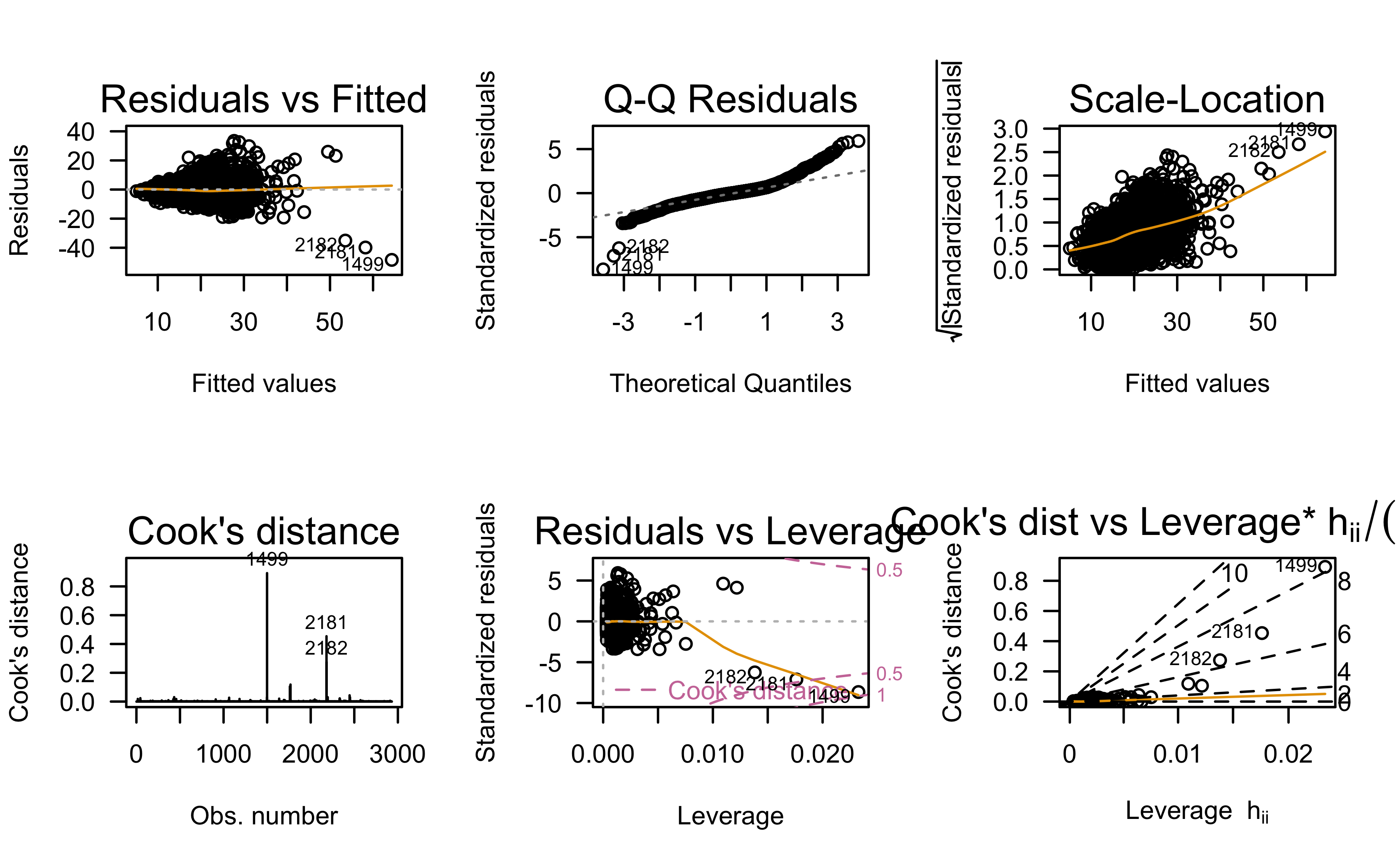
What assumptions appear to be in violation?
Let’s try a log transformation
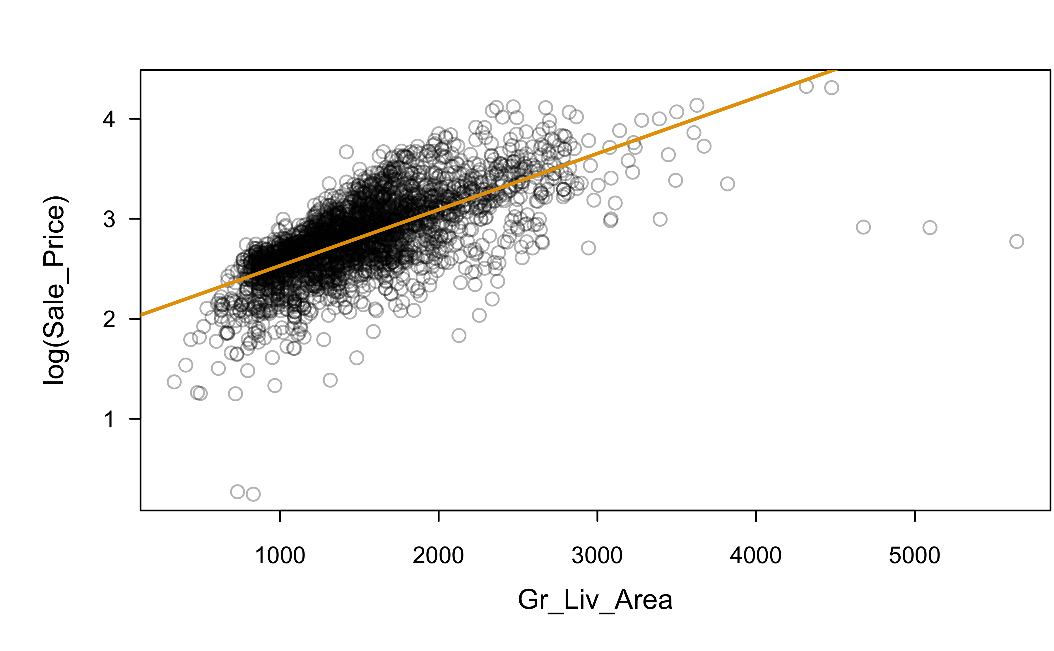
log(Sale_Price) ~ Gr_Liv_Area
Residual analysis:
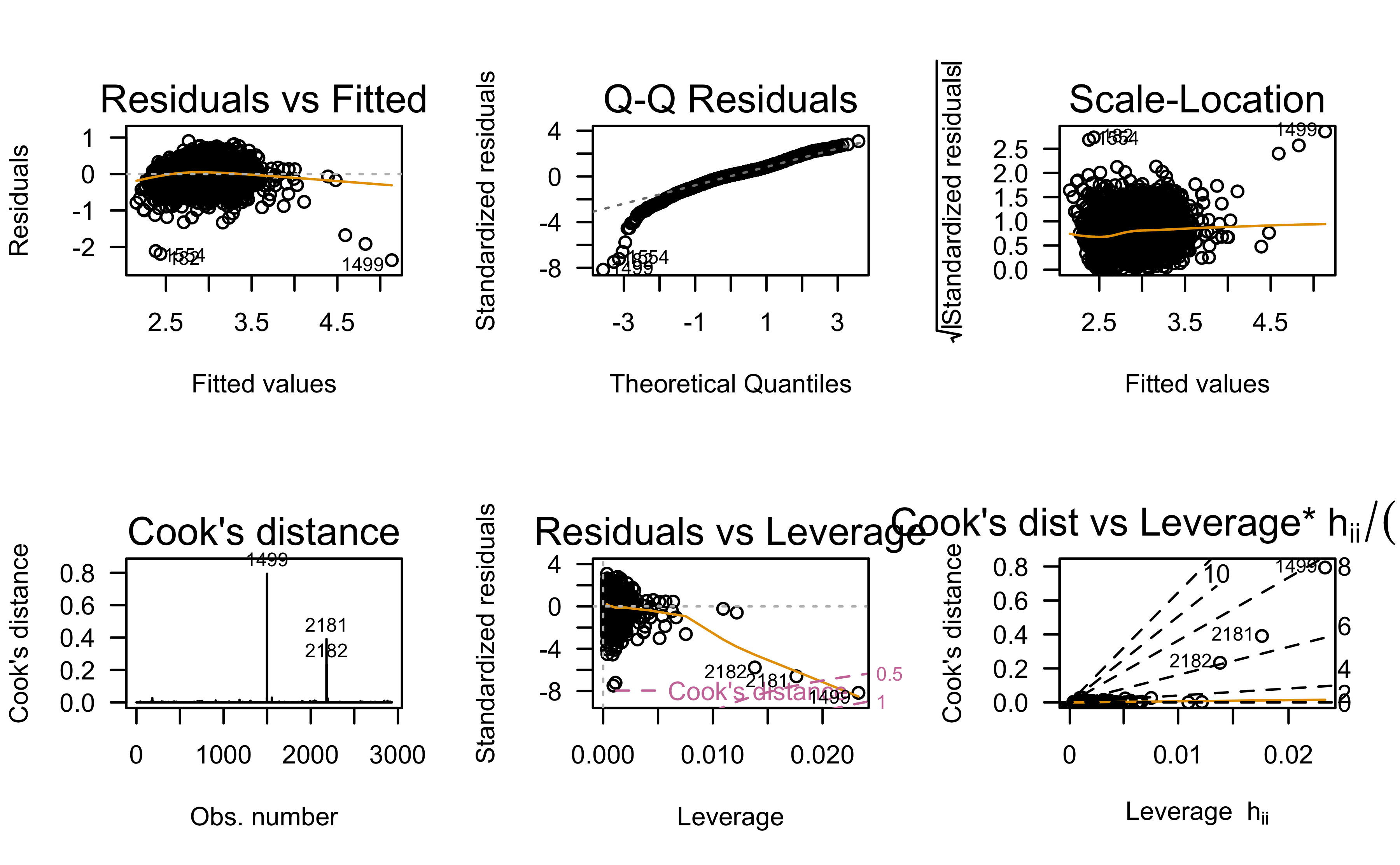
Any better?
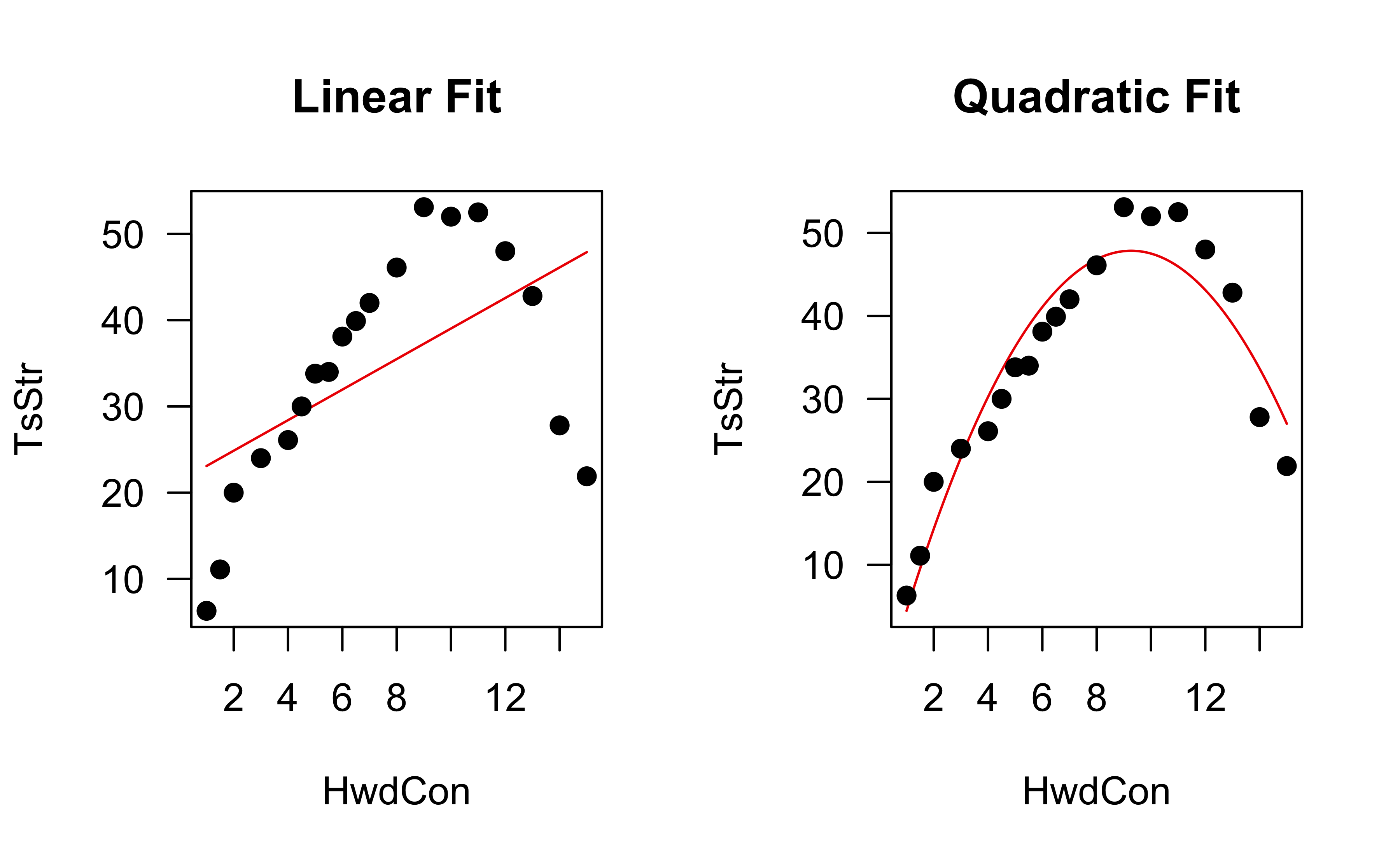
Example: paper strength data
Data concerning the strength of kraft paper and the percentage of hardwood in the batch of pulp from which the paper was produced.