Logistic Regression (Part II)

What’s going on with dibep?
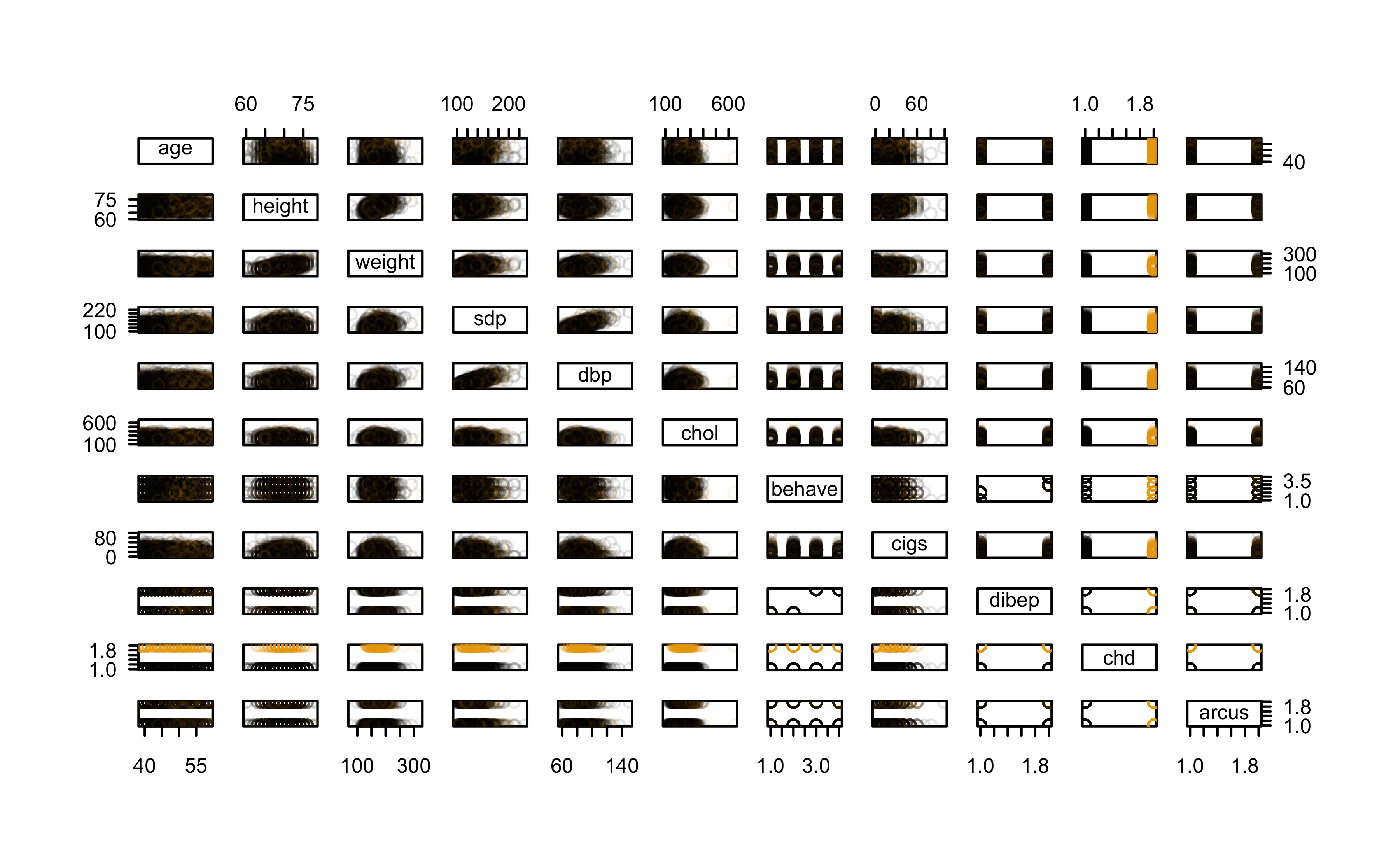
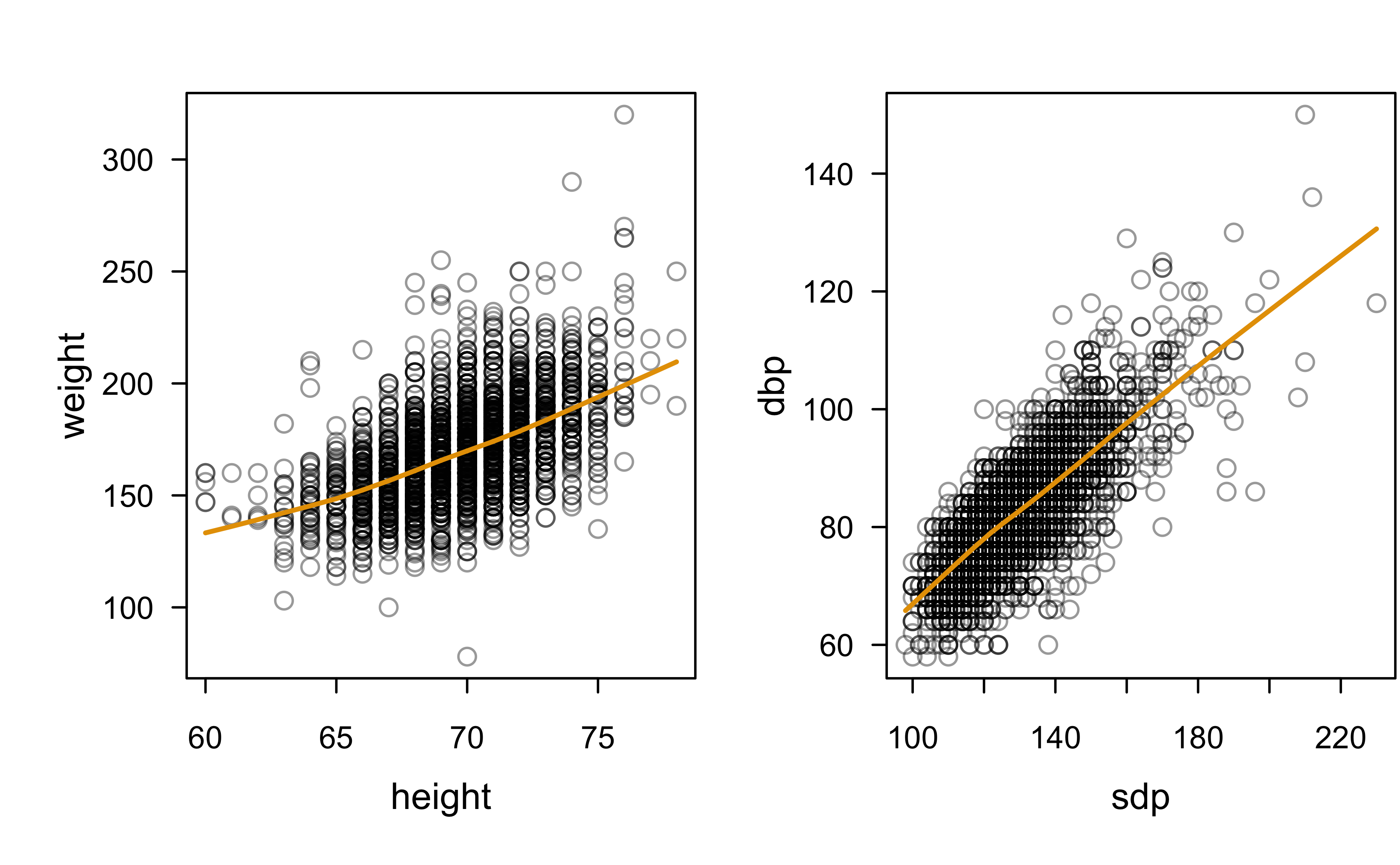
Let’s inspect the data a bit more; we’ll start with a SPLOM
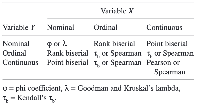
Measures of Association: How to Choose?1
Check pairwise correlations
Only looking at numeric columns:
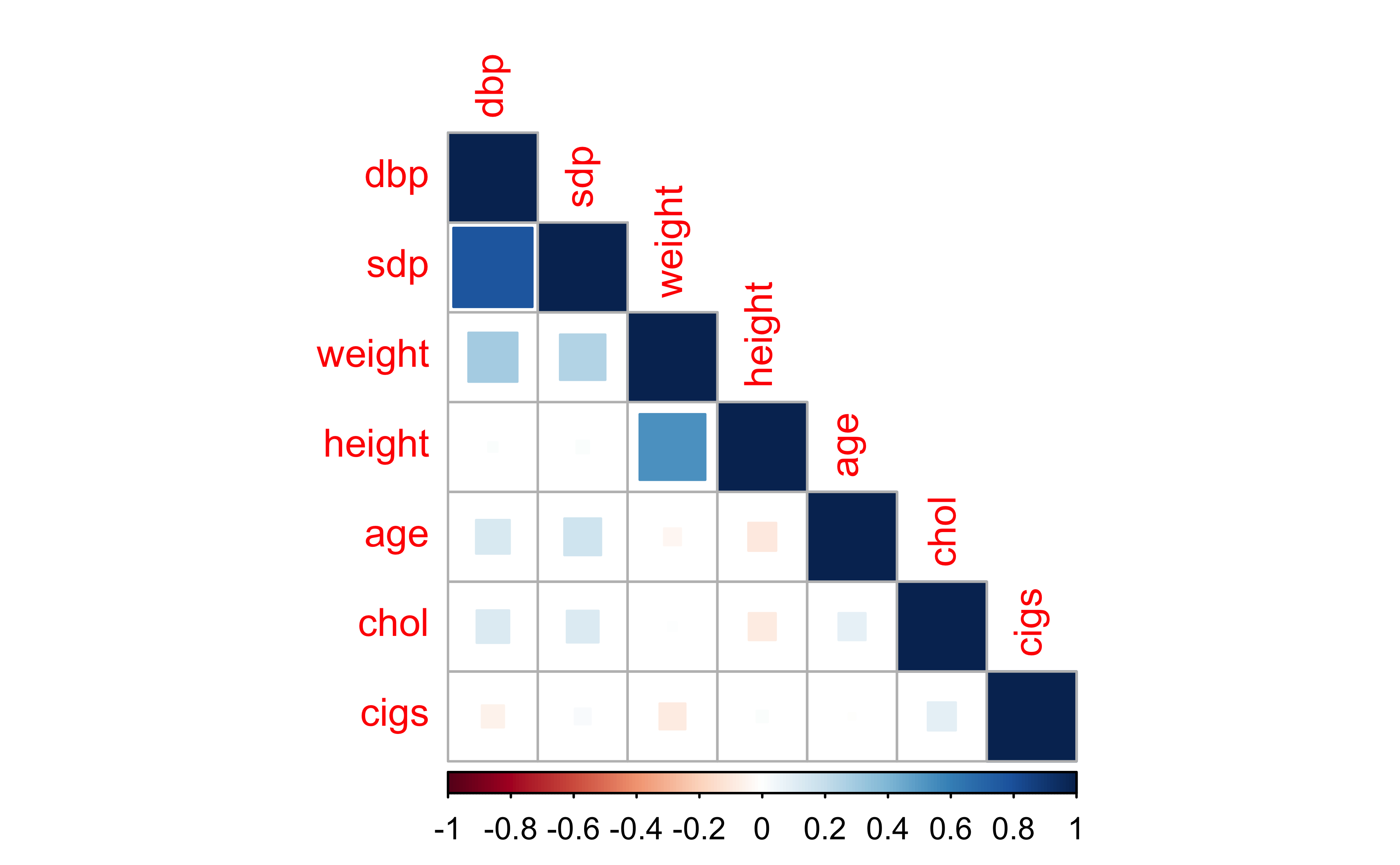
Check pairwise correlations
Pairwise scatterplots with LOWESS smoothers:
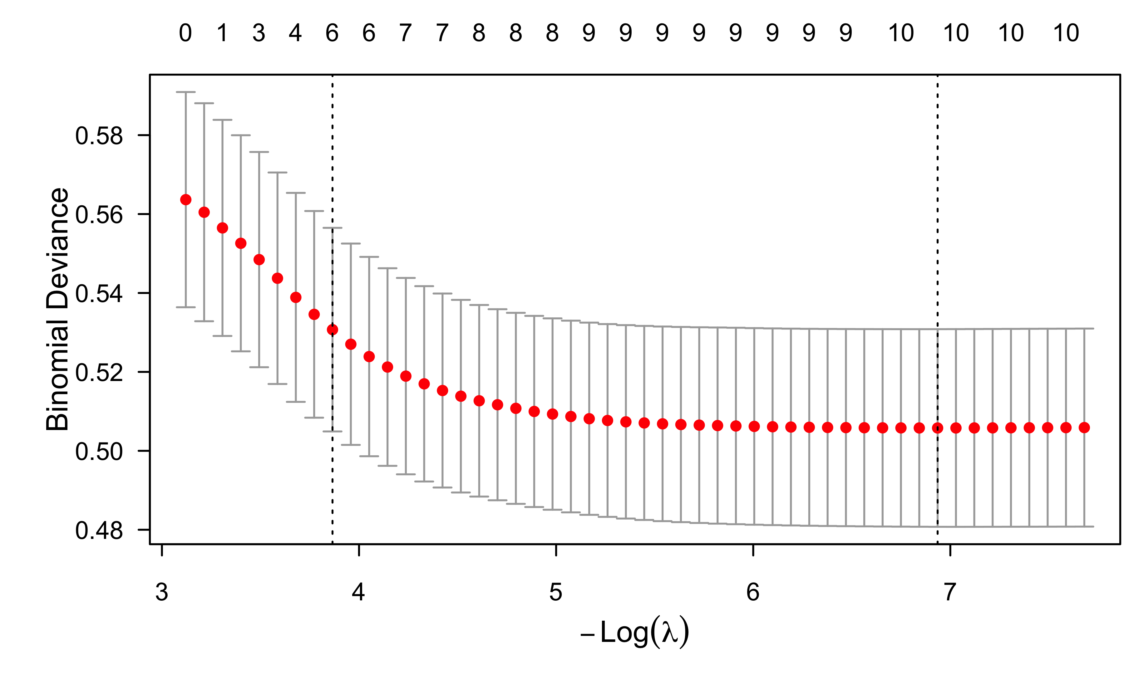
ENet fit to wcgs data
Show R code
library(glmnet)

# Fit an elastic net model (i.e., LASSO and ridge penalties) using 5-fold CV
wcgs.complete <- na.omit(wcgs)
X <- model.matrix(~. - chd - dibep - bmi - 1 , data = wcgs.complete)
#lr.enet <- cv.glmnet(X, y = ifelse(wcgs.complete$chd == "yes", 1, 0),
#                     family = "binomial", nfold = 5, keep = TRUE)
lr.enet <- glmnet(X, y = ifelse(wcgs.complete$chd == "yes", 1, 0),
                  family = "binomial")
plot(lr.enet, label = TRUE, xvar = "lambda")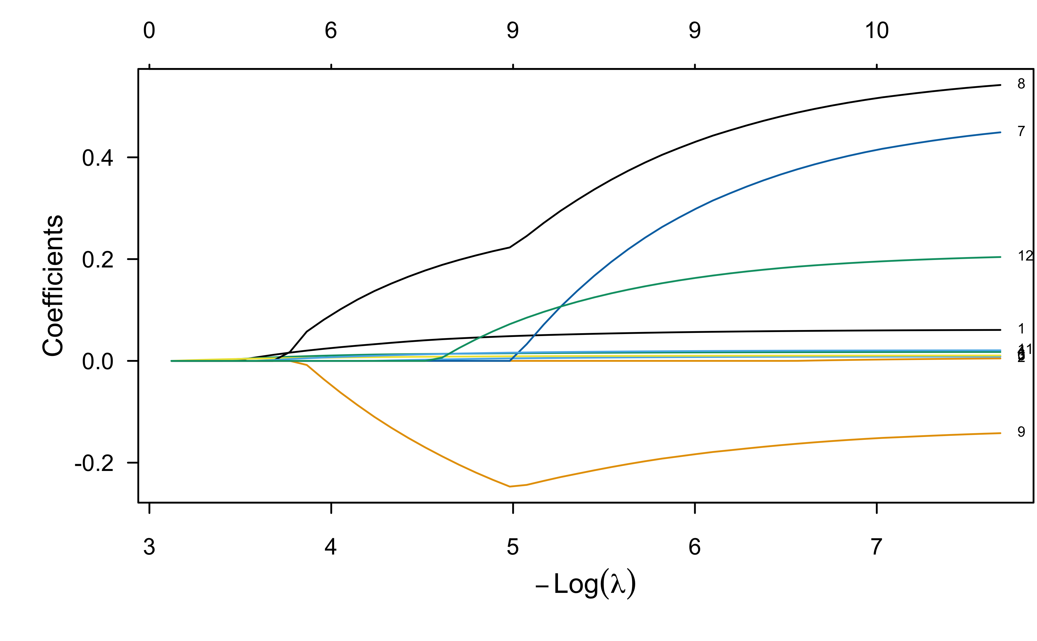
ENet fit to wcgs data
Classification boundary
Perfect seperation (or discrimination):
Show R code
# Simulate some data
N <- 200
d1 <- cbind(matrix(MASS::mvrnorm(2*N, mu = c(0, 0), Sigma = diag(2)), ncol = 2), 0)
d2 <- cbind(matrix(MASS::mvrnorm(2*N, mu = c(8, 8), Sigma = diag(2)), ncol = 2), 1)
d <- as.data.frame(rbind(d1, d2))
names(d) <- c("x1", "x2", "y")

# Fit a logistic regression
fit <- glm(y ~ ., data = d, family = binomial)

# Plot decision boundary using 0.5 threshold
pfun <- function(object, newdata) {
  prob <- predict(object, newdata = newdata, type = "response")
  label <- ifelse(prob > 0.5, 1, 0)  # force into class label
  label
}
plot(x2 ~ x1, data = d, col = d$y + 1)
treemisc::decision_boundary(fit, train = d, y = "y", x1 = "x1", x2 = "x2",
                            pfun = pfun, grid.resolution = 999)
legend("topleft", legend = c("y = 0", "y = 1"), col = c(1, 2), pch = 1)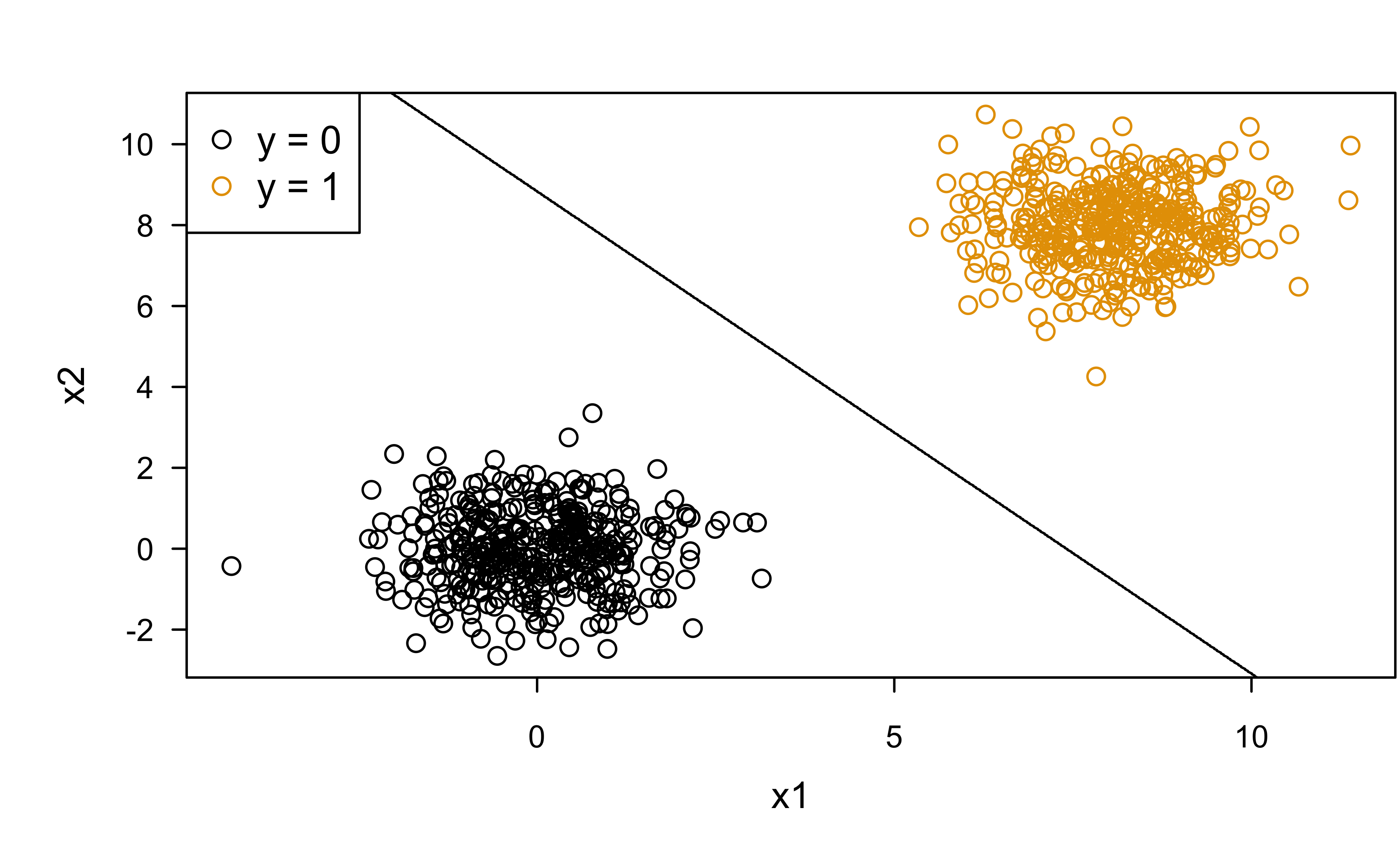
Classification boundary
Class overlap (four possibilities in terms of classification):
Show R code
# Simulate some data
N <- 200
d1 <- cbind(matrix(MASS::mvrnorm(2*N, mu = c(0, 0), Sigma = diag(2)), ncol = 2), 0)
d2 <- cbind(matrix(MASS::mvrnorm(2*N, mu = c(2, 2), Sigma = diag(2)), ncol = 2), 1)
d <- as.data.frame(rbind(d1, d2))
names(d) <- c("x1", "x2", "y")

# Fit a logistic regression
fit <- glm(y ~ ., data = d, family = binomial)

# Plot decision boundary using 0.5 threshold
pfun <- function(object, newdata) {
  prob <- predict(object, newdata = newdata, type = "response")
  label <- ifelse(prob > 0.5, 1, 0)  # force into class label
  label
}
plot(x2 ~ x1, data = d, col = d$y + 1)
treemisc::decision_boundary(fit, train = d, y = "y", x1 = "x1", x2 = "x2",
                            pfun = pfun, grid.resolution = 999)
legend("topleft", legend = c("y = 0", "y = 1"), col = c(1, 2), pch = 1)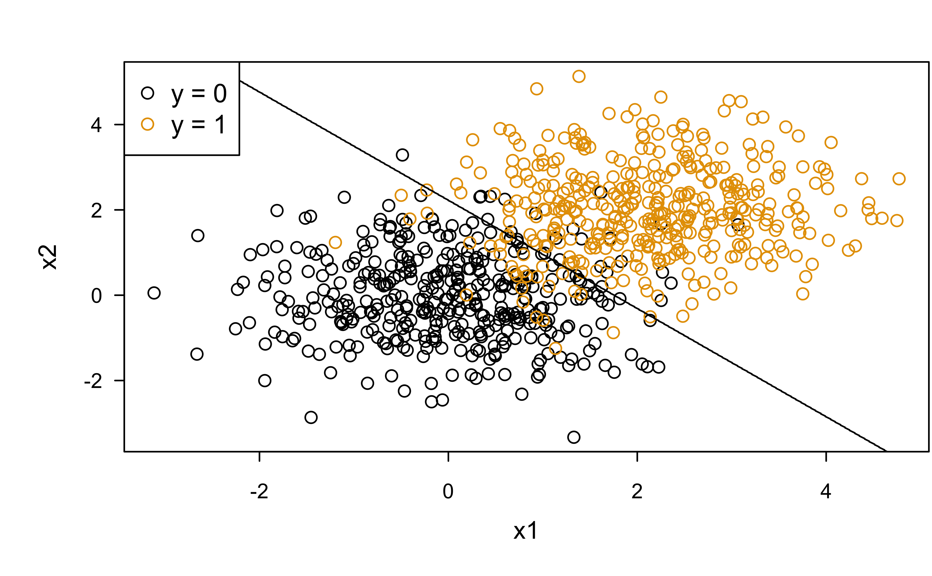
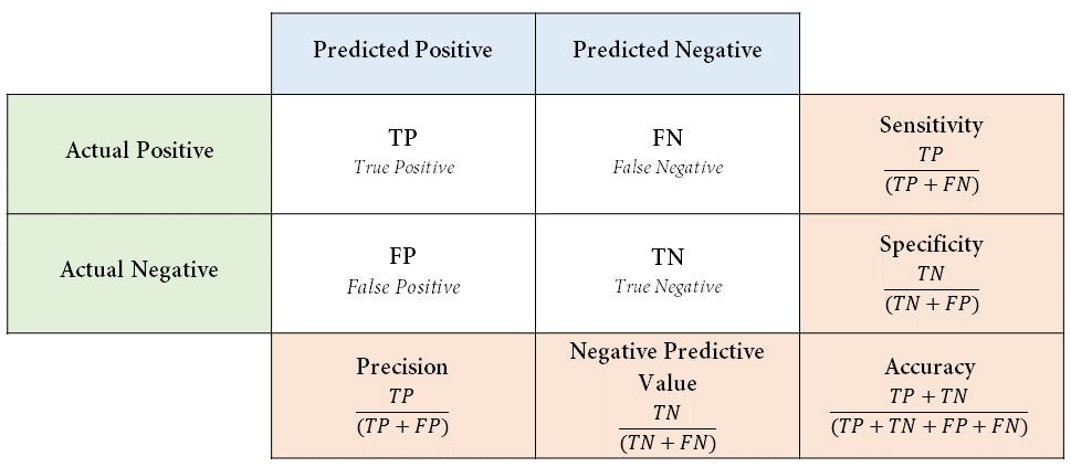
Confusion matrix
ROC curve (by hand)
Show R code
threshold <- seq(from = 0, to = 1, length = 999)
tp <- tn <- fp <- fn <- numeric(length(threshold))
for (i in seq_len(length(threshold))) {
  classes <- ifelse(prob > threshold[i], "yes", "no")
  tp[i] <- sum(classes == "yes" & y == "yes")  # true positives
  tn[i] <- sum(classes == "no"  & y == "no")  # true negatives
  fp[i] <- sum(classes == "yes" & y == "no")  # false positives
  fn[i] <- sum(classes == "no"  & y == "yes")  # false negatives
}
tpr <- tp / (tp + fn)  # sensitivity
tnr <- tn / (tn + fp)  # specificity

# Plot ROC curve
plot(tnr, y = tpr, type = "l", col = 2, lwd = 2, xlab = "TNR (or specificity)",
     ylab = "TPR (or sensitivity)")
abline(1, -1, lty = 2)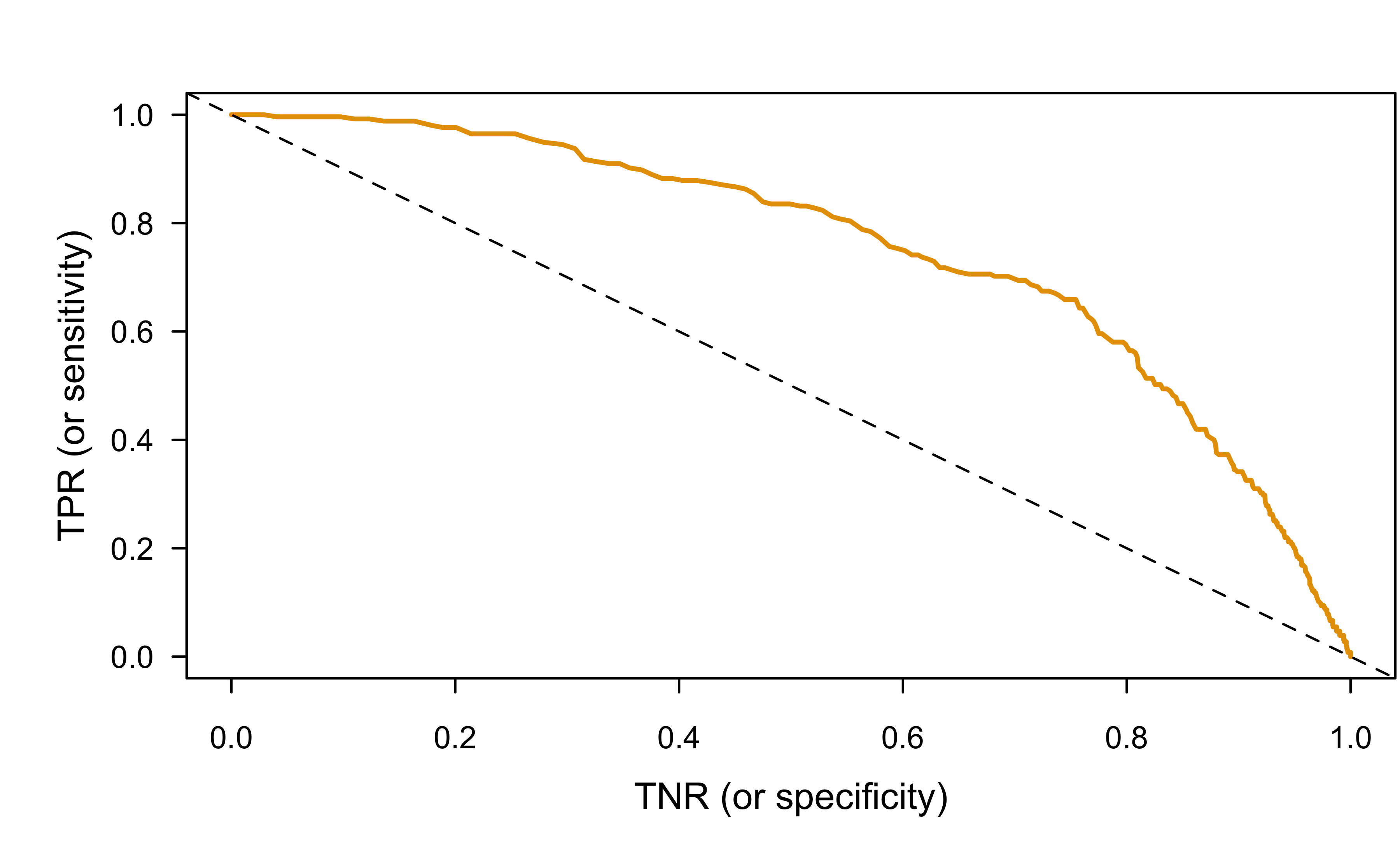
ROC curve (pROC package)
Can be useful to use a package sometimes (e.g., for computing are under the ROC curve; AKA AUROC or AUC)
Call:
roc.default(response = y, predictor = prob)

Data: prob in 2885 controls (y no) < 255 cases (y yes).
Area under the curve: 0.751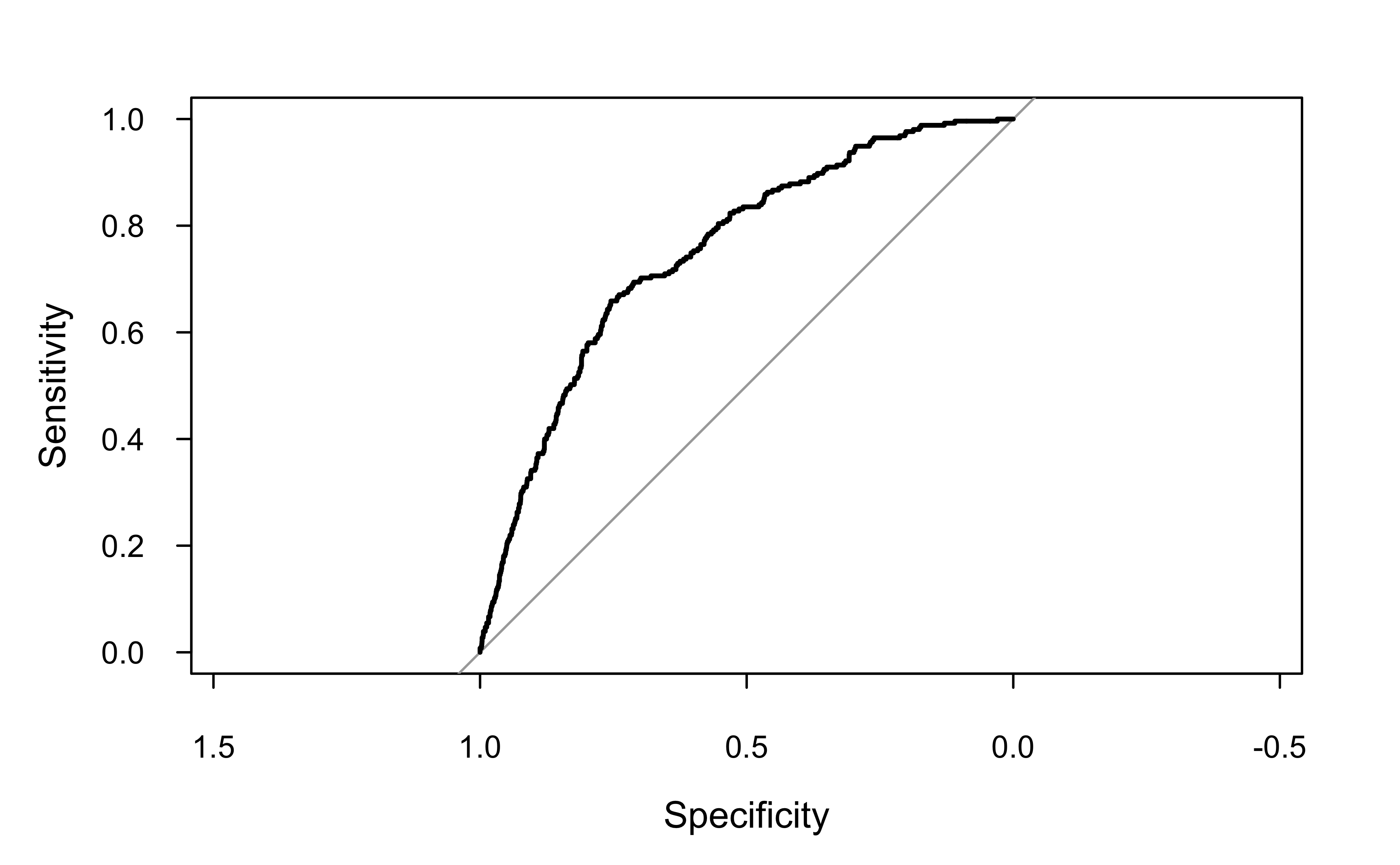
LOCO scores for wcgs example
Show R code
Call:
glm(formula = chd ~ ., family = binomial, data = wcgs)

Coefficients:
               Estimate Std. Error z value Pr(>|z|)
(Intercept)  -1.168e+01  1.026e+00 -11.387  < 2e-16 ***
age           5.922e-02  1.233e-02   4.804 1.56e-06 ***
sdp           1.806e-02  6.435e-03   2.807   0.0050 **
dbp          -3.193e-04  1.087e-02  -0.029   0.9766
chol          1.047e-02  1.520e-03   6.889 5.64e-12 ***
behaveA2      8.498e-02  2.229e-01   0.381   0.7030
behaveB3     -6.238e-01  2.449e-01  -2.547   0.0109 *
behaveB4     -4.994e-01  3.211e-01  -1.555   0.1199
cigs          2.139e-02  4.294e-03   4.982 6.31e-07 ***
arcuspresent  2.238e-01  1.437e-01   1.558   0.1193
bmi           5.880e-02  2.717e-02   2.164   0.0305 *
---
Signif. codes:  0 '***' 0.001 '**' 0.01 '*' 0.05 '.' 0.1 ' ' 1

(Dispersion parameter for binomial family taken to be 1)

    Null deviance: 1769.2  on 3139  degrees of freedom
Residual deviance: 1572.3  on 3129  degrees of freedom
  (14 observations deleted due to missingness)
AIC: 1594.3

Number of Fisher Scoring iterations: 6
Show R code
# Leave-one-covariate-out (LOCO) method
#
# Note: Would be better to incorporate some form of cross-validation (or bootstrap)
x.names <- attr(fit$terms, "term.labels")
loco <- numeric(length(x.names))
baseline <- deviance(fit)  # smaller is better; could also use AUROC, Brier score, etc.
loco <- sapply(x.names, FUN = function(x.name) {
  wcgs.copy <- wcgs
  wcgs.copy[[x.name]] <- NULL
  fit.new <- glm(chd ~ ., data = wcgs.copy, family = binomial(link = "logit"))
  deviance(fit.new) - baseline  # measure drop in performance
})
names(loco) <- x.names
sort(loco, decreasing = TRUE)
chol cigs age behave arcus sdp
5.201189e+01 2.385372e+01 2.298085e+01 2.233397e+01 1.203822e+01 7.647463e+00
bmi dbp
4.630518e+00 8.624341e-04 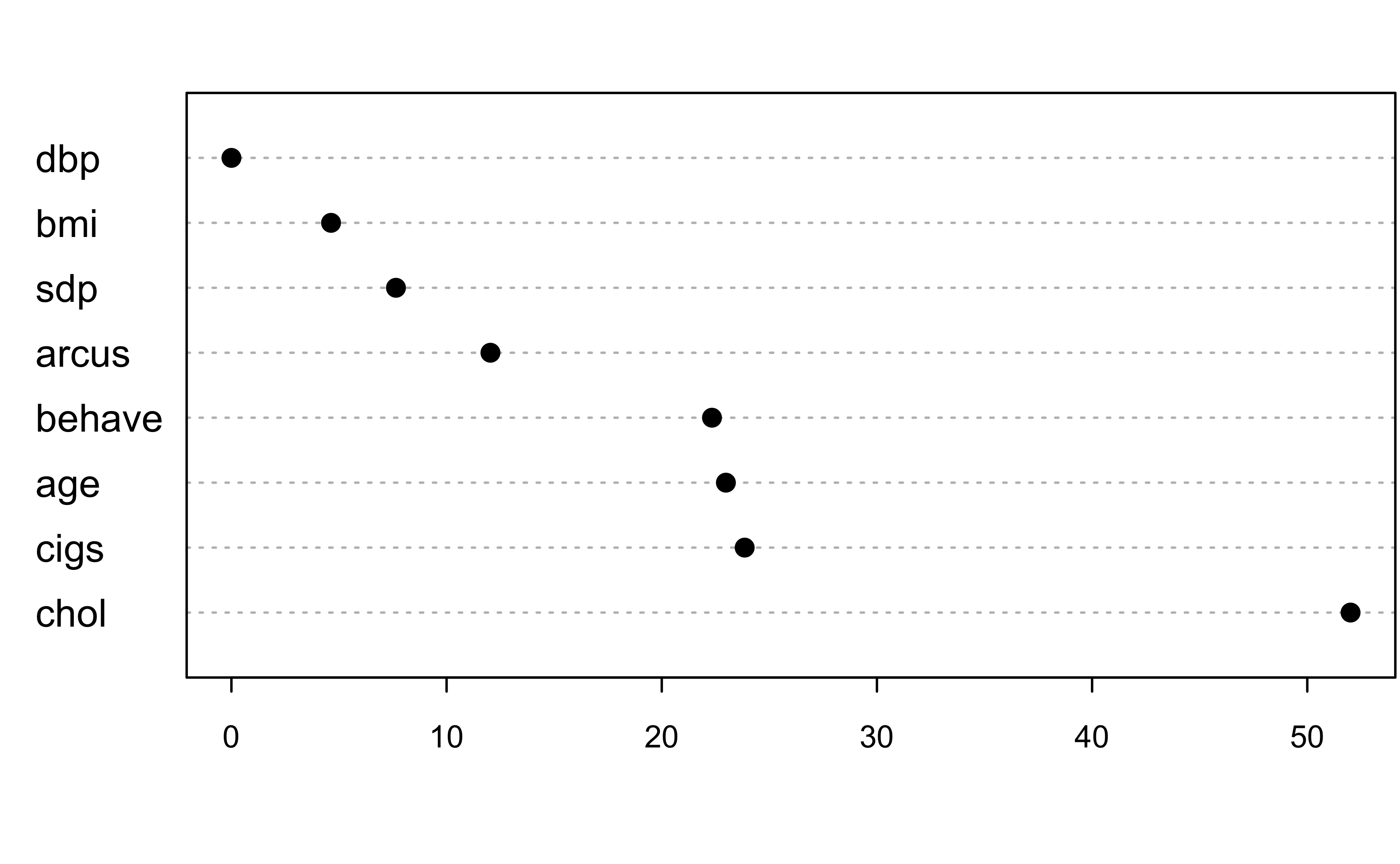
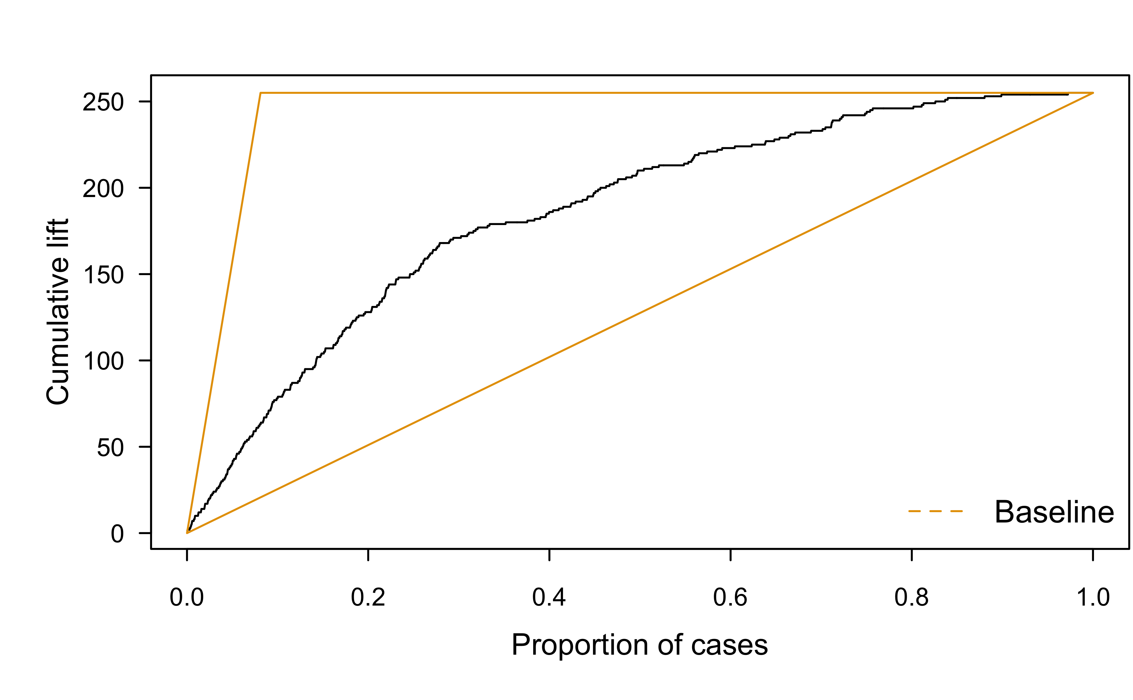
Lift charts
Cumulative gains chart applied to wcgs example (lr.fit.all):
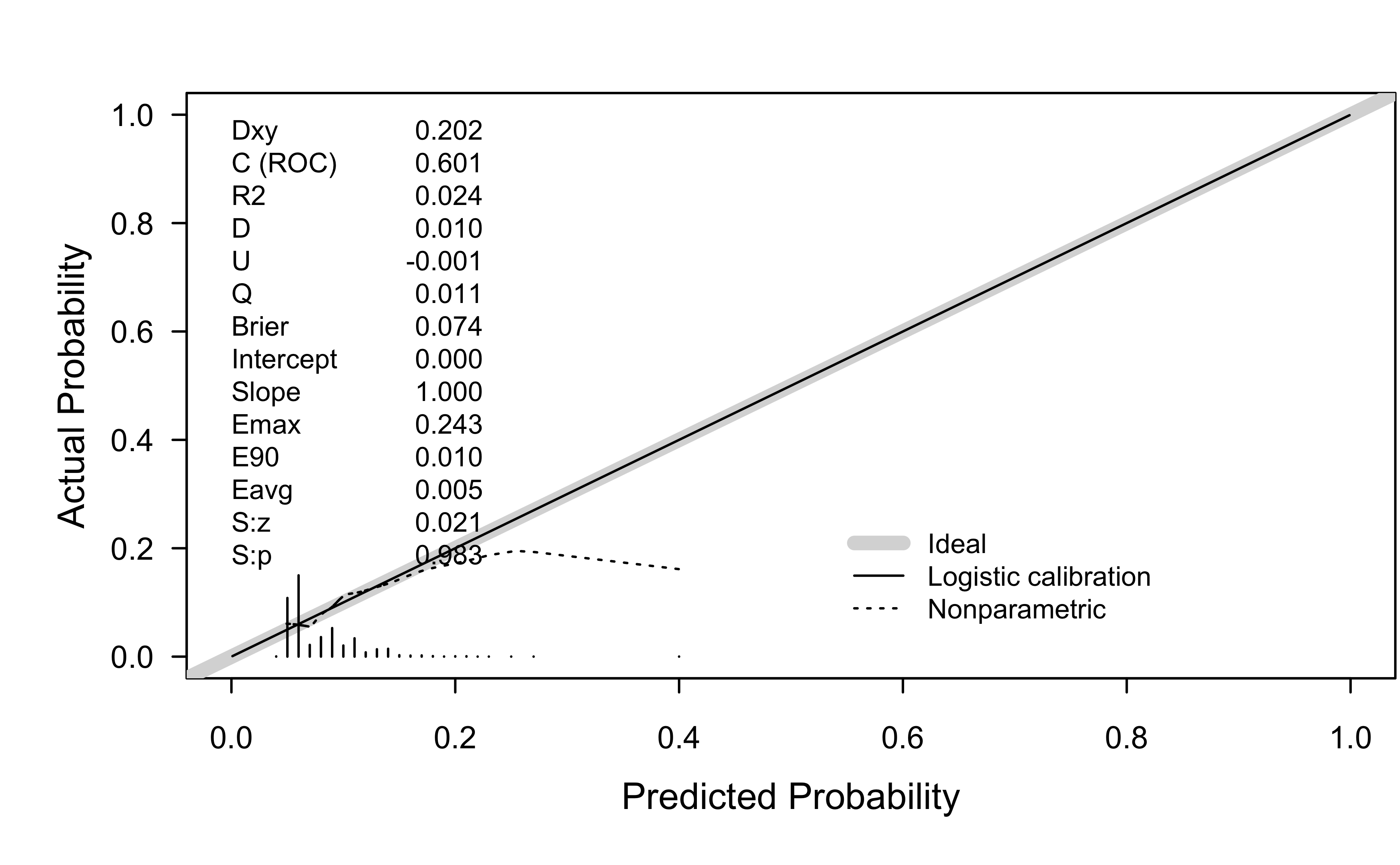
Probability calibration
The rms function val.prob() can be used for this: