Logistic Regression (Part III)

Brandon M. Greenwell, PhD

University of Cincinnati

Variations of logistic regression

Logistic regression

• In logistic regression, we use the logit: \[ \text{logit}\left(p\right) = \boldsymbol{x}^\top\boldsymbol{\beta} = \eta \] which results in \[ p = \left[1 + \exp\left(-\eta\right)\right]^{-1} = F\left(\eta\right) \]

• Technically, \(F\) can be any monotonic function that maps \(\eta\) to \(\left[0, 1\right]\) (e.g., any CDF will work)

• \(F^{-1}\) is called the link function

The probit model

• The probit model uses \(F\left(\eta\right) = \Phi\left(\eta\right)\) (i.e., the CDF of a standard normal distribution) \[ P\left(Y = 1 | \boldsymbol{x}\right) = \Phi\left(\beta_0 + \beta_1x_1 + \cdots\right) = \Phi\left(\boldsymbol{x}^\top\boldsymbol{\beta}\right) \]

• \(F^{-1} = \Phi^{-1}\) is called the probit link, which yields \[ \text{probit}\left(p\right) = \Phi^{-1}\left(p\right) = \boldsymbol{x}^\top\boldsymbol{\beta} \]

• The term probit is short for probability unit

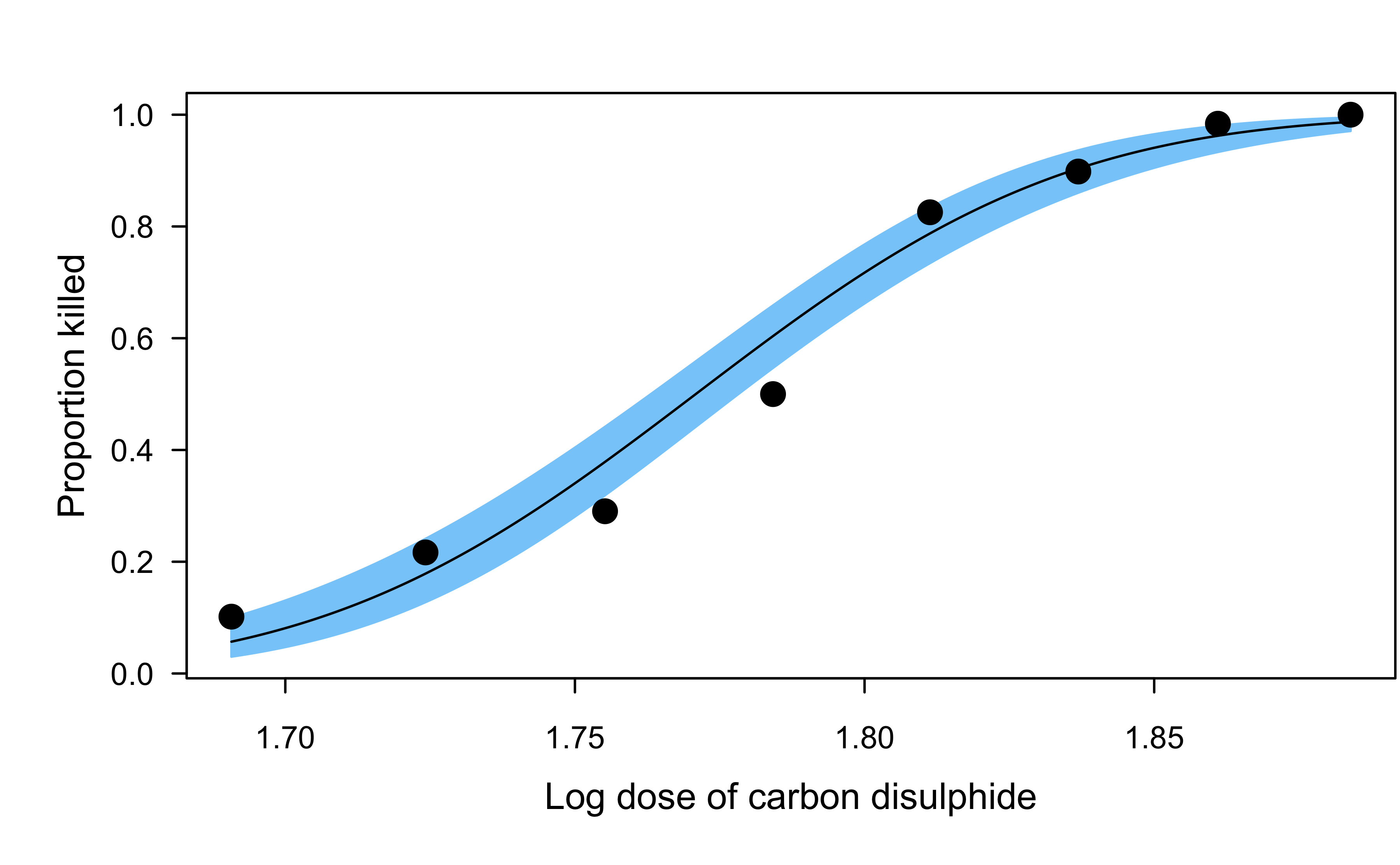
• Proposed in Bliss (1934) and still common for modeling dose-response relationships

Dobson’s beetle data

The data give the number of flour beetles killed after five hour exposure to the insecticide carbon disulphide at eight different concentrations.

beetle <- investr::beetle
fit <- glm(cbind(y, n-y) ~ ldose, data = beetle, 
           family = binomial(link = "probit"))
investr::plotFit(
  fit, pch = 19, cex = 1.2, lwd = 2, 
  xlab = "Log dose of carbon disulphide", ylab = "Proportion killed",
  interval = "confidence", shade = TRUE, col.conf = "lightskyblue"
)

Other link functions

Common link function for binary regression include:

• Logit (most common and the default an most software)
• Probit (next most common)
• Log-log
• Complimentary log-log
• Cauchit

Application to wcgs data set

Comparing coefficients from different link functions:

wcgs <- na.omit(subset(faraway::wcgs, select = -c(typechd, timechd, behave)))

# Fit binary GLMs with different link functions
fit.logit <- glm(chd ~ ., data = wcgs, family = binomial(link = "logit"))
fit.probit <- glm(chd ~ ., data = wcgs, family = binomial(link = "probit"))
fit.cloglog <- glm(chd ~ ., data = wcgs, family = binomial(link = "cloglog"))
fit.cauchit <- glm(chd ~ ., data = wcgs, family = binomial(link = "cauchit"))

# Compare coefficients
coefs <- cbind(
  "logit" = coef(fit.logit),
  "probit" = coef(fit.probit),
  "cloglog" = coef(fit.cloglog),
  "cauchit" = coef(fit.cauchit)
)
round(coefs, digits = 3)

               logit probit cloglog cauchit
(Intercept)  -12.246 -6.452 -11.377 -24.086
age            0.062  0.031   0.057   0.115
height         0.007  0.003   0.007   0.053
weight         0.009  0.005   0.007   0.003
sdp            0.018  0.010   0.017   0.042
dbp           -0.001 -0.001  -0.001  -0.001
chol           0.011  0.006   0.010   0.020
cigs           0.021  0.011   0.019   0.043
dibepB        -0.658 -0.341  -0.604  -1.320
arcuspresent   0.211  0.101   0.206   0.711

Application to wcgs data set

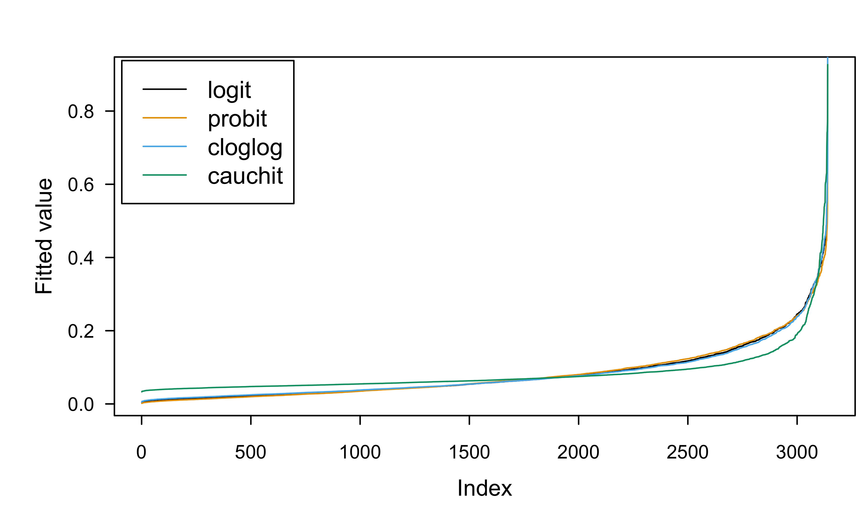
Comparing fitted values from different link functions:

# Compare fitted values (i.e., predicted probabilities)
preds <- cbind(
  "logit" = fitted(fit.logit),
  "probit" = fitted(fit.probit),
  "cloglog" = fitted(fit.cloglog),
  "cauchit" = fitted(fit.cauchit)
)
head(round(preds, digits = 3))

  logit probit cloglog cauchit
1 0.071  0.072   0.072   0.076
2 0.073  0.074   0.075   0.084
3 0.010  0.006   0.011   0.038
4 0.010  0.006   0.012   0.039
5 0.169  0.167   0.168   0.150
6 0.034  0.033   0.035   0.051

Application to wcgs data set

Comparing fitted values from different link functions:

plot(sort(preds[, "logit"]), type = "l", ylab = "Fitted value")
lines(sort(preds[, "probit"]), col = 2)
lines(sort(preds[, "cloglog"]), col = 3)
lines(sort(preds[, "cauchit"]), col = 4)
legend("topleft", legend = c("logit", "probit", "cloglog", "cauchit"), 
       col = 1:4, lty = 1, inset = 0.01)

As a latent variable model

• Logistic regression (and the other link functions) has an equivalent formulation as a latent variable model

• Consider a linear model with continuous outcome \(Y^\star = \boldsymbol{x}^\top\boldsymbol{\beta} + \epsilon\)

• Imagine that we can only observe the binary variable \[ Y = \begin{cases} 1 \quad \text{if } Y^\star > 0, \\ 0 \quad \text{otherwise} \end{cases} \]

• Assuming \(\epsilon \sim \text{Logistic}\left(0, 1\right)\) leads to the usual logit model

• Assuming \(\epsilon \sim N\left(0, 1\right)\) leads to the probit model

• And so on…

Application: surrogate residual

• There are several types of residuals defined for logistic regression (e.g., deviance residuals and Pearson residuals)
• The surrogate residual act like the usual residual from a normal linear model and has similar properties!
• See Liu and Zhang (2018), Greenwell et al. (2018), and Cheng et al. (2020) for details
• A novel R-squared measure based on the surrogate idea was proposed in Liu et al. (2022)
• For implementation, see R packages sure, SurrogateRsq, and PAsso

Binomial data

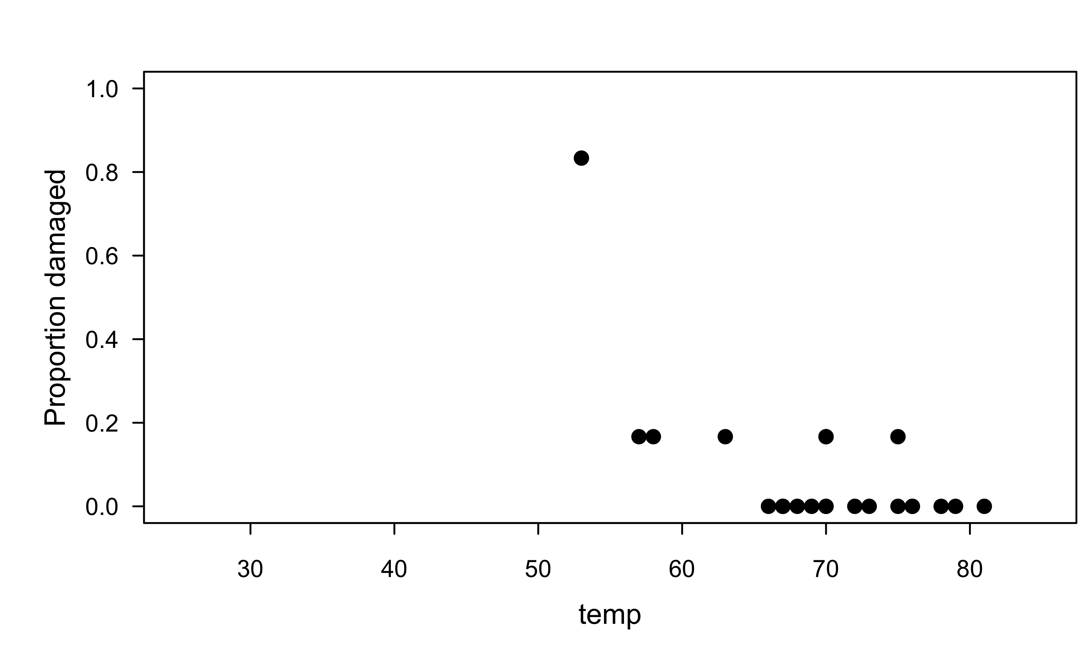
O-rings example

On January 28, 1986, the Space Shuttle Challenger broke apart 73 seconds into its flight, killing all seven crew members aboard. The crash was linked to the failure of O-ring seals in the rocket engines. Data was collected on the 23 previous shuttle missions. The launch temperature on the day of the crash was 31 \(^\circ\)F.

head(orings <- faraway::orings)

O-rings example

plot(damage/6 ~ temp, data = orings, xlim = c(25, 85), pch = 19,
     ylim = c(0, 1), ylab = "Proportion damaged")

O-rings example

Expand binomial data into independent Bernoulli trials

tmp <- rep(orings$temp, each = 6)
dmg <- sapply(orings$damage, FUN = function(x) rep(c(0, 1), times = c(6 - x, x)))
orings2 <- data.frame("temp" = tmp, "damage" = as.vector(dmg))
head(orings2, n = 15)

O-rings example

Here we’ll just fit a logistic regression to the expanded bernoulli version of the data

# Fit a logistic regression (LR) model using 0/1 version of the data
orings.lr <- glm(damage ~ temp, data = orings2, 
                 family = binomial(link = "logit"))
summary(orings.lr)

Call:
glm(formula = damage ~ temp, family = binomial(link = "logit"), 
    data = orings2)

Coefficients:
            Estimate Std. Error z value Pr(>|z|)    
(Intercept) 11.66299    3.29616   3.538 0.000403 ***
temp        -0.21623    0.05318  -4.066 4.77e-05 ***
---
Signif. codes:  0 '***' 0.001 '**' 0.01 '*' 0.05 '.' 0.1 ' ' 1

(Dispersion parameter for binomial family taken to be 1)

    Null deviance: 76.745  on 137  degrees of freedom
Residual deviance: 54.759  on 136  degrees of freedom
AIC: 58.759

Number of Fisher Scoring iterations: 6

O-rings example

What’s the estimated probability that an O-ring will be damaged at 31 \(^\circ\)F? Give a point estimate as well as a 95% confidence interval.

predict(orings.lr, newdata = data.frame("temp" = 31), type = "response", 
        se = TRUE)

$fit
        1 
0.9930342 

$se.fit
         1 
0.01153302 

$residual.scale
[1] 1

# Better approach for a 95% CI?
pred <- predict(orings.lr, newdata = data.frame("temp" = 31), 
                type = "link", se = TRUE)
plogis(pred$fit + c(-qnorm(0.975), qnorm(0.975)) * pred$se.fit)

[1] 0.8444824 0.9997329

O-rings example

# Is this extrapolating?
plot(damage / 6 ~ temp, data = orings, pch = 19, cex = 1.3,
     col = adjustcolor(1, alpha.f = 0.3), xlim = c(0, 100), ylim = c(0, 1))
x <- seq(from = 0, to = 100, length = 1000)
y <- predict(orings.lr, newdata = data.frame("temp" = x), 
             type = "response")
lines(x, y, lwd = 2, col = 2)
abline(v = 31, lty = 2, col = 3)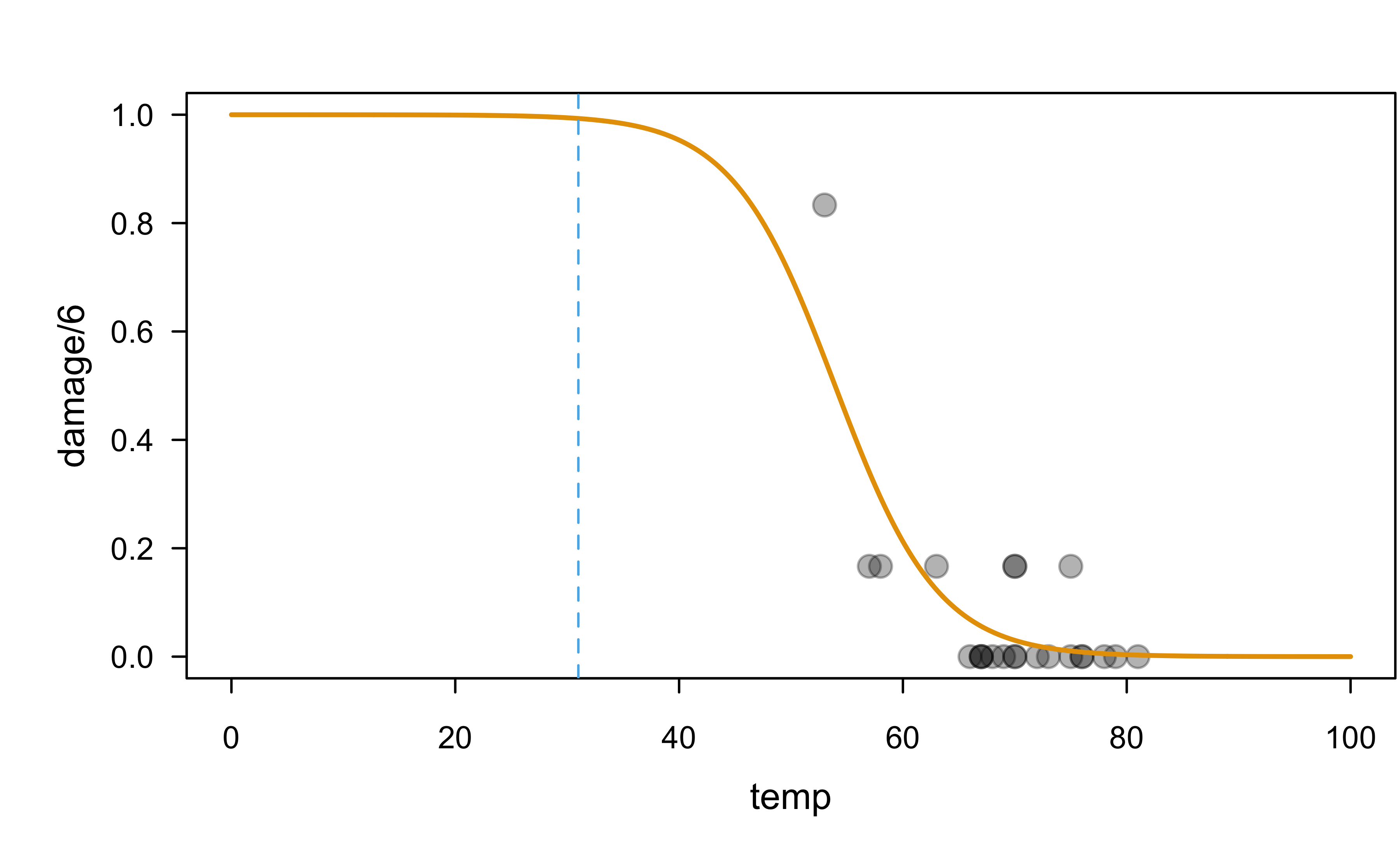

O-rings examples

More interesting question: at what temperature(s) can we expect the risk/probability of damage to exceed 0.8?

This is a problem of inverse estimation, which is the purpose of the investr package!

# To install from CRAN, use
#
# > install.packages("investr")
#
# See ?investr::invest for details and examples
investr::invest(orings.lr, y0 = 0.8, interval = "Wald", lower = 40, upper = 60)

 estimate     lower     upper        se 
47.525881 39.993462 55.058299  3.843141 

O-rings example

Here’s an equivalent logistic regression model fit to the original binomial version of the data (need to provide number of successes and number of failures)

orings.lr2 <- glm(cbind(damage, 6 - damage) ~ temp, data = orings,
                  family = binomial(link = "logit"))
summary(orings.lr2)

Call:
glm(formula = cbind(damage, 6 - damage) ~ temp, family = binomial(link = "logit"), 
    data = orings)

Coefficients:
            Estimate Std. Error z value Pr(>|z|)    
(Intercept) 11.66299    3.29626   3.538 0.000403 ***
temp        -0.21623    0.05318  -4.066 4.78e-05 ***
---
Signif. codes:  0 '***' 0.001 '**' 0.01 '*' 0.05 '.' 0.1 ' ' 1

(Dispersion parameter for binomial family taken to be 1)

    Null deviance: 38.898  on 22  degrees of freedom
Residual deviance: 16.912  on 21  degrees of freedom
AIC: 33.675

Number of Fisher Scoring iterations: 6

Overdispersion

Overdispersion

• For a Bernoulli random variable \(Y\), \(E(Y) = p\) and \(V(Y) = p(1 - p)\).

• Sometimes the data exhibit variance greater than expected. Adding a dispersion parameter makes the model more flexible: \(V(Y) = \sigma^2 p(1 - p)\).

• Overdispersion occurs when variability exceeds expectations under the response distribution. Underdispersion is less common.

Overdispersion

• For a correctly specified model, the Pearson chi-square statistic and deviance, divided by their degrees of freedom, should be about one. Values much larger indicate overdispersion.

• Such goodness-of-fit statistics require replicated data. Problems like outliers, wrong link function, omitted terms, or untransformed predictors can inflate goodness-of-fit statistics.

• A large difference between the Pearson statistic and deviance suggests data sparsity.

O-rings example

You can check for overdispersion manually or by using performance:

performance::check_overdispersion(orings.lr2)

# Overdispersion test

 dispersion ratio = 1.206
          p-value = 0.616

Overdispersion

Two common (but equivalent) ways to handle overdispersion in R:

1. Estimate the dispersion parameter \(\sigma^2\) and provide it to summary() to adjust the standard errors approriately

2. Use the quasibinomial() family

Overdispersion

Estimate the dispersion parameter \(\sigma^2\); analagous to MSE in linear regression

(sigma2 <- sum(residuals(orings.lr2, type = "pearson") ^ 2) / orings.lr2$df.residual)

[1] 1.336542

# Print model summary based on estimated dispersion parameter
summary(orings.lr2, dispersion = sigma2)

Call:
glm(formula = cbind(damage, 6 - damage) ~ temp, family = binomial(link = "logit"), 
    data = orings)

Coefficients:
            Estimate Std. Error z value Pr(>|z|)    
(Intercept) 11.66299    3.81077   3.061 0.002209 ** 
temp        -0.21623    0.06148  -3.517 0.000436 ***
---
Signif. codes:  0 '***' 0.001 '**' 0.01 '*' 0.05 '.' 0.1 ' ' 1

(Dispersion parameter for binomial family taken to be 1.336542)

    Null deviance: 38.898  on 22  degrees of freedom
Residual deviance: 16.912  on 21  degrees of freedom
AIC: 33.675

Number of Fisher Scoring iterations: 6

Overdispersion

Can use quasibinomial() family to account for over-dispersion automatically (notice the estimated coeficients don’t change)

orings.qb <- glm(cbind(damage, 6 - damage) ~ temp, data = orings, 
                 family = quasibinomial)
summary(orings.qb)

Call:
glm(formula = cbind(damage, 6 - damage) ~ temp, family = quasibinomial, 
    data = orings)

Coefficients:
            Estimate Std. Error t value Pr(>|t|)   
(Intercept) 11.66299    3.81077   3.061  0.00594 **
temp        -0.21623    0.06148  -3.517  0.00205 **
---
Signif. codes:  0 '***' 0.001 '**' 0.01 '*' 0.05 '.' 0.1 ' ' 1

(Dispersion parameter for quasibinomial family taken to be 1.336542)

    Null deviance: 38.898  on 22  degrees of freedom
Residual deviance: 16.912  on 21  degrees of freedom
AIC: NA

Number of Fisher Scoring iterations: 6

Generalized additive models (GAMs)

• \(\text{logit}\left(p\right) = \beta_0 + f_1\left(x_1\right) + f_2\left(x_2\right) + \dots + f_p\left(x_p\right)\)

  • The \(f_i\) are referred to as shape functions or term contributions and are often modeled using splines

  • Can also include pairwise interactions of the form \(f_{ij}\left(x_i, x_j\right)\)

• Easy to interpret (e.g., just plot the individual shape functions)!

  • Interaction effects can be understood with heat maps, etc.

• Modern GAMs, called GA²Ms, automatically include relevant pairwise interaction effects

Explainable boosting machines (EBMs)

• EBM ≈ .darkblue[GA²M] + .green[Boosting] + .tomato[Bagging]
• Python library: interpret

Questions?