Regression for Multinomial and Ordinal Outcomes

Brandon M. Greenwell, PhD

University of Cincinnati

Regression for Multinomial Outcomes

Multinomial data

• The multinomial distribution is an extension of the binomial where the outcome can take on more than two values

• The categories can be nominal (e.g., have no natural ordering) or ordinal in nature (e.g., low < medium < high)

• We’ll start with the case of a nominal outcome having more than two categories

• Let \(Y\) be a discrete r.v. that can take on one of \(J\) categories with \(\left\{\mathrm{P}\left(Y = j\right) = p_j\right\}_{j=1}^J\), where \(\sum_{j=1}^Jp_j=1\)

Multinomial logit model

• Similar to binary regression, we need a way to link the probabilities \(p_j\) to the predictors \(\boldsymbol{x} = \left(x_1, x_2, \dots, x_p\right)^\top\)

• Need to ensure each \(0 \le p_j \le 1\) and that \(\sum_{j=1}^Jp_j = 1\)

• Idea is similar to fitting several logistic regressions using one of the categories as the reference or baseline (say, \(j = 1\))

• To that end, we define the \(J-1\) logits \(\eta_j = \boldsymbol{x}^\top\boldsymbol{\beta}_j = \log\left(p_j / p_1\right)\), where \(j \ne 1\)

• Notice we have a set of coefficients for each comparison!

Multinomial logit model

• To ensure \(\sum_{j=1}^Jp_j = 1\), we have \[ p_i = \frac{\exp\left(\eta_i\right)}{1 + \sum_{j=2}^J\exp\left(\eta_j\right)} \]

• This implies that \(p_1 = 1 - \sum_{j=2}^Jp_j\)

1996 National Election Study

1996 National Election Study

• We’ll consider a sample taken from a subset of the 1996 American National Election Study

• Contained in the nes96 data frame in the faraway 📦

str(nes96 <- faraway::nes96)

'data.frame':   944 obs. of  10 variables:
 $ popul : int  0 190 31 83 640 110 100 31 180 2800 ...
 $ TVnews: int  7 1 7 4 7 3 7 1 7 0 ...
 $ selfLR: Ord.factor w/ 7 levels "extLib"<"Lib"<..: 7 3 2 3 5 3 5 5 4 3 ...
 $ ClinLR: Ord.factor w/ 7 levels "extLib"<"Lib"<..: 1 3 2 4 6 4 6 4 6 3 ...
 $ DoleLR: Ord.factor w/ 7 levels "extLib"<"Lib"<..: 6 5 6 5 4 6 4 5 3 7 ...
 $ PID   : Ord.factor w/ 7 levels "strDem"<"weakDem"<..: 7 2 2 2 1 2 2 5 4 1 ...
 $ age   : int  36 20 24 28 68 21 77 21 31 39 ...
 $ educ  : Ord.factor w/ 7 levels "MS"<"HSdrop"<..: 3 4 6 6 6 4 4 4 4 3 ...
 $ income: Ord.factor w/ 24 levels "$3Kminus"<"$3K-$5K"<..: 1 1 1 1 1 1 1 1 1 1 ...
 $ vote  : Factor w/ 2 levels "Clinton","Dole": 2 1 1 1 1 1 1 1 1 1 ...

1996 National Election Study

• For simplicity, we’ll consider three variables: age, education level, and income groups of each respondent

• Some of the factors are “ordered” by default; E.g., income (respondent’s education level):

levels(nes96$income)

 [1] "$3Kminus"   "$3K-$5K"    "$5K-$7K"    "$7K-$9K"    "$9K-$10K"  
 [6] "$10K-$11K"  "$11K-$12K"  "$12K-$13K"  "$13K-$14K"  "$14K-$15K" 
[11] "$15K-$17K"  "$17K-$20K"  "$20K-$22K"  "$22K-$25K"  "$25K-$30K" 
[16] "$30K-$35K"  "$35K-$40K"  "$40K-$45K"  "$45K-$50K"  "$50K-$60K" 
[21] "$60K-$75K"  "$75K-$90K"  "$90K-$105K" "$105Kplus" 

• Same goes for PID and educ (respondent’s party identification and education, respectively)

1996 National Election Study

Here’s a cleaned up version of the data we’ll work with:

# Condense party identification (PID) column into three categories
party <- nes96$PID
levels(party) <- c(
  "Democrat", "Democrat",
  "Independent", "Independent", "Independent", 
  "Republican", "Republican"
)

# Convert income to numeric
inca <- c(1.5, 4, 6, 8, 9.5, 10.5, 11.5, 12.5, 13.5, 14.5, 16, 18.5, 21, 23.5,
          27.5, 32.5, 37.5, 42.5, 47.5, 55, 67.5, 82.5, 97.5, 115)
income <- inca[unclass(nes96$income)]

# Construct new data set for analysis
rnes96 <- data.frame(
  "party" = party, 
  "income" = income, 
  "education" = nes96$educ, 
  "age" = nes96$age
)

# Print summary of data set
summary(rnes96)

         party         income        education        age       
 Democrat   :380   Min.   :  1.50   MS    : 13   Min.   :19.00  
 Independent:239   1st Qu.: 23.50   HSdrop: 52   1st Qu.:34.00  
 Republican :325   Median : 37.50   HS    :248   Median :44.00  
                   Mean   : 46.58   Coll  :187   Mean   :47.04  
                   3rd Qu.: 67.50   CCdeg : 90   3rd Qu.:58.00  
                   Max.   :115.00   BAdeg :227   Max.   :91.00  
                                    MAdeg :127                  

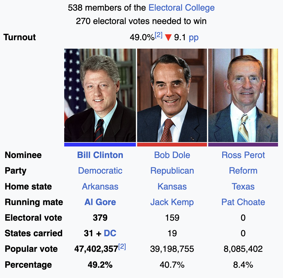
1996 National Election Study

Let’s continue with some visual exploration:

library(dplyr)
library(ggplot2)

theme_set(theme_bw())

# Aggregate data; what's happening here?
egp <- group_by(rnes96, education, party) %>% 
  summarise(count = n()) %>%
  group_by(education) %>% 
  mutate(etotal = sum(count), proportion = count/etotal)

# Plot results
ggplot(egp, aes(x = education, y = proportion, group = party, 
                linetype = party, color = party)) + 
  geom_line(size = 2)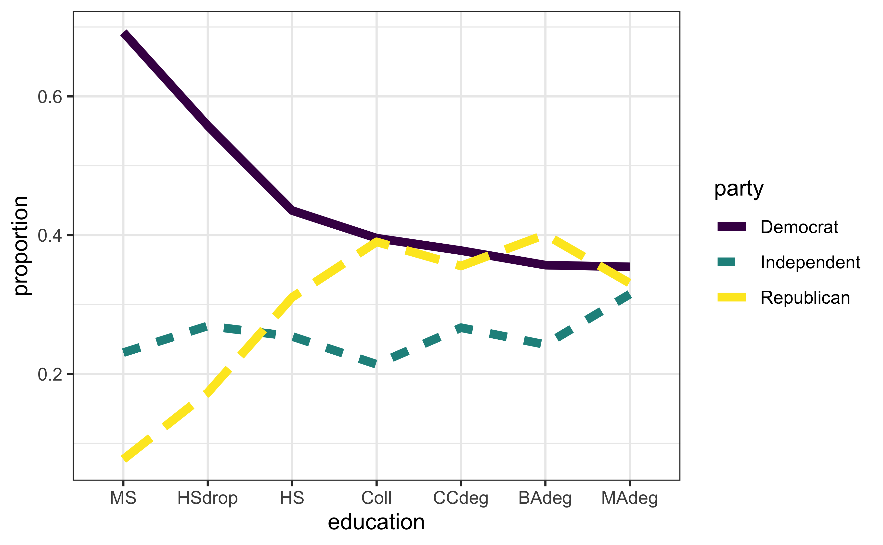

1996 National Election Study

Let’s continue with some visual exploration:

# Aggregate data; what's happening here?
igp <- mutate(rnes96, income_group = cut_number(income, 7)) %>% 
  group_by(income_group, party) %>% 
  summarise(count = n()) %>% 
  group_by(income_group) %>% 
  mutate(etotal = sum(count), proportion = count / etotal)

# Plot results
ggplot(igp, aes(x = income_group, y = proportion, group = party, 
                linetype = party, color = party)) +
  scale_x_discrete(guide = guide_axis(angle = 45)) +
  geom_line(size = 2)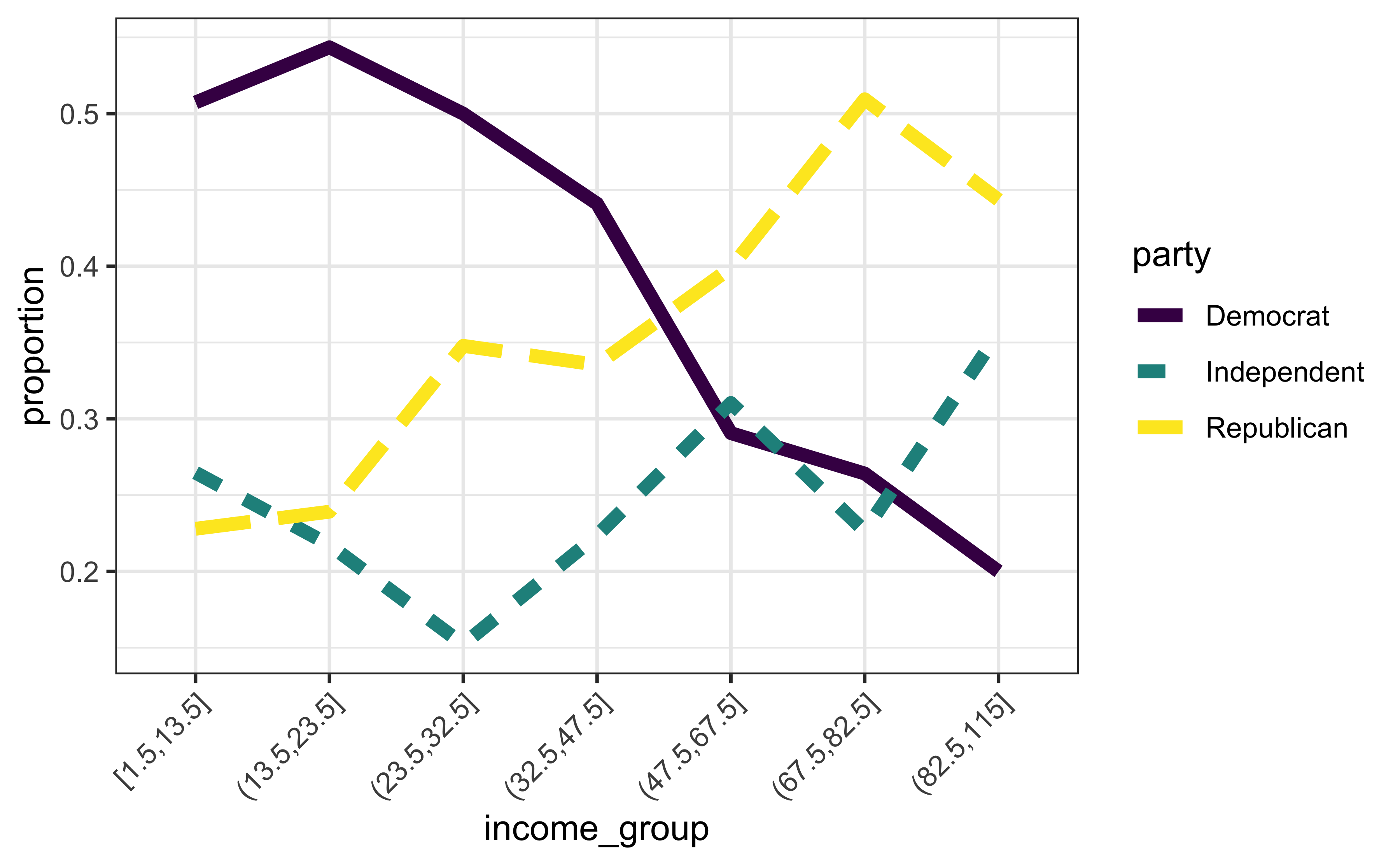

1996 National Election Study

Let’s continue with some visual exploration:

# Aggregate data; what's happening here?
agp <- rnes96 %>% 
  group_by(age, party) %>% 
  summarise(count = n()) %>% 
  group_by(age) %>% 
  mutate(etotal = sum(count), proportion = count / etotal)

# Plot results
ggplot(agp, aes(x = age, y = proportion, group = party, 
                linetype = party, color = party)) +
  geom_line(size = 1, alpha = 0.5)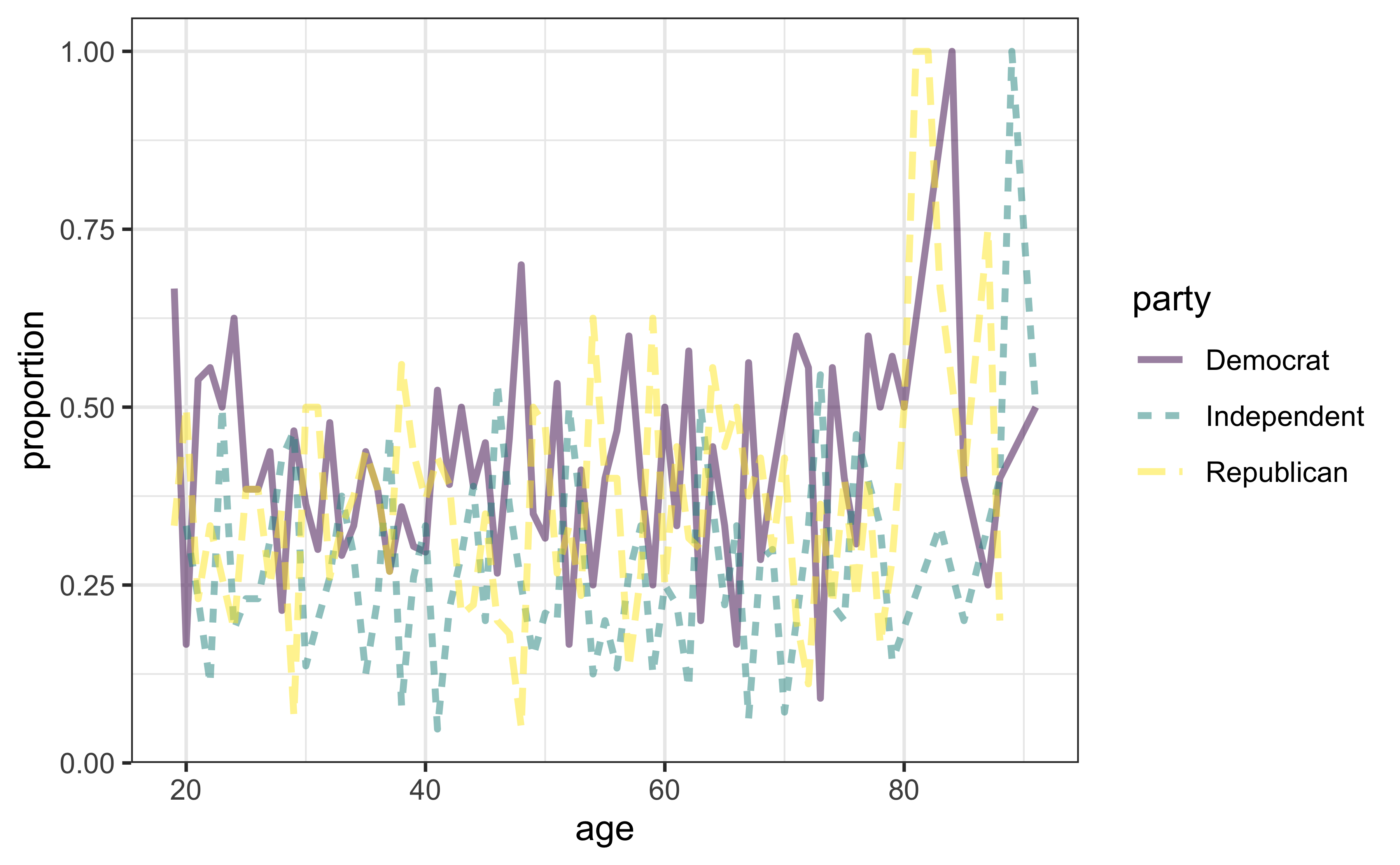

1996 National Election Study

Define the following probabilities:

• \(p_{d} = P\left(\text{voting democrat}\right)\);
• \(p_{i} = P\left(\text{voting independent}\right)\);
• \(p_{r} = P\left(\text{voting republican}\right)\),

where \(p_d + p_i + p_r = 1\). Assume for now that income is the only independent variable of interest.

1996 National Election Study

The multinomial logit model effectively fits several logits (one for every class except the baseline, which is arbitrary; here, it’s democrat):

• \(\log\left(p_{i} / p_{d}\right) = \beta_0 + \beta_1 \mathtt{income}\quad\) (log odds of voting independent vs. democrat);
• \(\log\left(p_{r} / p_{d}\right) = \alpha_0 + \alpha_1 \mathtt{income}\quad\) (log odds of voting republican vs. democrat).

Here we use \(\beta_i\) and \(\alpha_i\) to remind us that the estimated coefficients between the two logits will be different.

1996 National Election Study

Multinomial logit model using all three predictors:

library(nnet)  # install.packages("nnet")

(mfit <- multinom(party ~ age + education + income, data = rnes96, trace = FALSE))

Call:
multinom(formula = party ~ age + education + income, data = rnes96, 
    trace = FALSE)

Coefficients:
            (Intercept)          age education.L education.Q education.C
Independent   -1.197260 0.0001534525  0.06351451  -0.1217038   0.1119542
Republican    -1.642656 0.0081943691  1.19413345  -1.2292869   0.1544575
            education^4 education^5 education^6     income
Independent -0.07657336   0.1360851  0.15427826 0.01623911
Republican  -0.02827297  -0.1221176 -0.03741389 0.01724679

Residual Deviance: 1968.333 
AIC: 2004.333 

Brief digression…

• By default, R encodes ordered factors using orthogonal polynomials

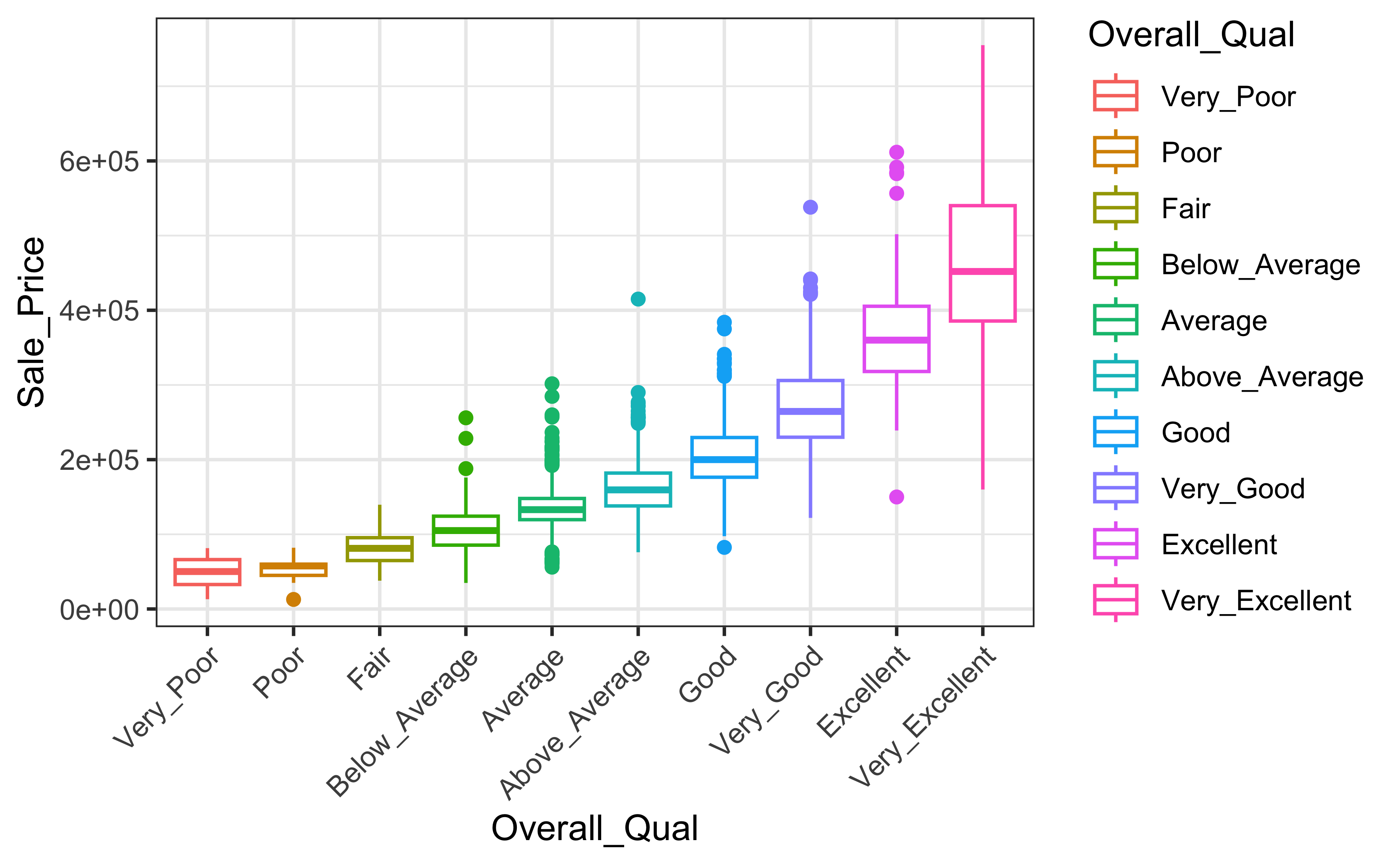
• Ames Housing example:

ames <- AmesHousing::make_ames()
ggplot(ames, aes(x = Overall_Qual, y = Sale_Price)) +#log(Sale_Price))) +
  geom_boxplot(aes(color = Overall_Qual)) +
  scale_x_discrete(guide = guide_axis(angle = 45)) 

1996 National Election Study

No \(p\)-values here!

summary(mfit)

Call:
multinom(formula = party ~ age + education + income, data = rnes96, 
    trace = FALSE)

Coefficients:
            (Intercept)          age education.L education.Q education.C
Independent   -1.197260 0.0001534525  0.06351451  -0.1217038   0.1119542
Republican    -1.642656 0.0081943691  1.19413345  -1.2292869   0.1544575
            education^4 education^5 education^6     income
Independent -0.07657336   0.1360851  0.15427826 0.01623911
Republican  -0.02827297  -0.1221176 -0.03741389 0.01724679

Std. Errors:
            (Intercept)         age education.L education.Q education.C
Independent   0.3265951 0.005374592   0.4571884   0.4142859   0.3498491
Republican    0.3312877 0.004902668   0.6502670   0.6041924   0.4866432
            education^4 education^5 education^6      income
Independent   0.2883031   0.2494706   0.2171578 0.003108585
Republican    0.3605620   0.2696036   0.2031859 0.002881745

Residual Deviance: 1968.333 
AIC: 2004.333 

1996 National Election Study

• How do we interpret the coefficients? How about for income?

• All else held constant, for every ⚠️one-unit increase in income⚠️, the multinomial log odds of voting republican, relative to democrat increase by 0.017.

• Gross… 🤢

• Effect plots to the rescue!

1996 National Election Study

Look at predicted probabilities:

head(probs <- predict(mfit, type = "probs"))

   Democrat Independent Republican
1 0.5923052   0.1975326  0.2101622
2 0.5919378   0.1687055  0.2393567
3 0.5970789   0.1732058  0.2297154
4 0.5924809   0.1719775  0.2355417
5 0.5423563   0.1583973  0.2992464
6 0.5907590   0.1683954  0.2408456

# Sanity check
head(rowSums(probs))

1 2 3 4 5 6 
1 1 1 1 1 1 

1996 National Election Study

library(pdp)  # for partial dependence (PD) plots

# Compute partial dependence of party identification on income
pfun <- function(object, newdata) {
  probs <- predict(object, newdata = newdata, type = "probs")
  colMeans(probs)  # return average probability for each class
}
pd.inc <- partial(mfit, pred.var = "income", pred.fun = pfun)
ggplot(pd.inc, aes(x = income, y = yhat, linetype = yhat.id, color = yhat.id)) +
  geom_line(size = 2) +
  xlab("Income group midpoint (in thousands)") +
  ylab("Partial dependence")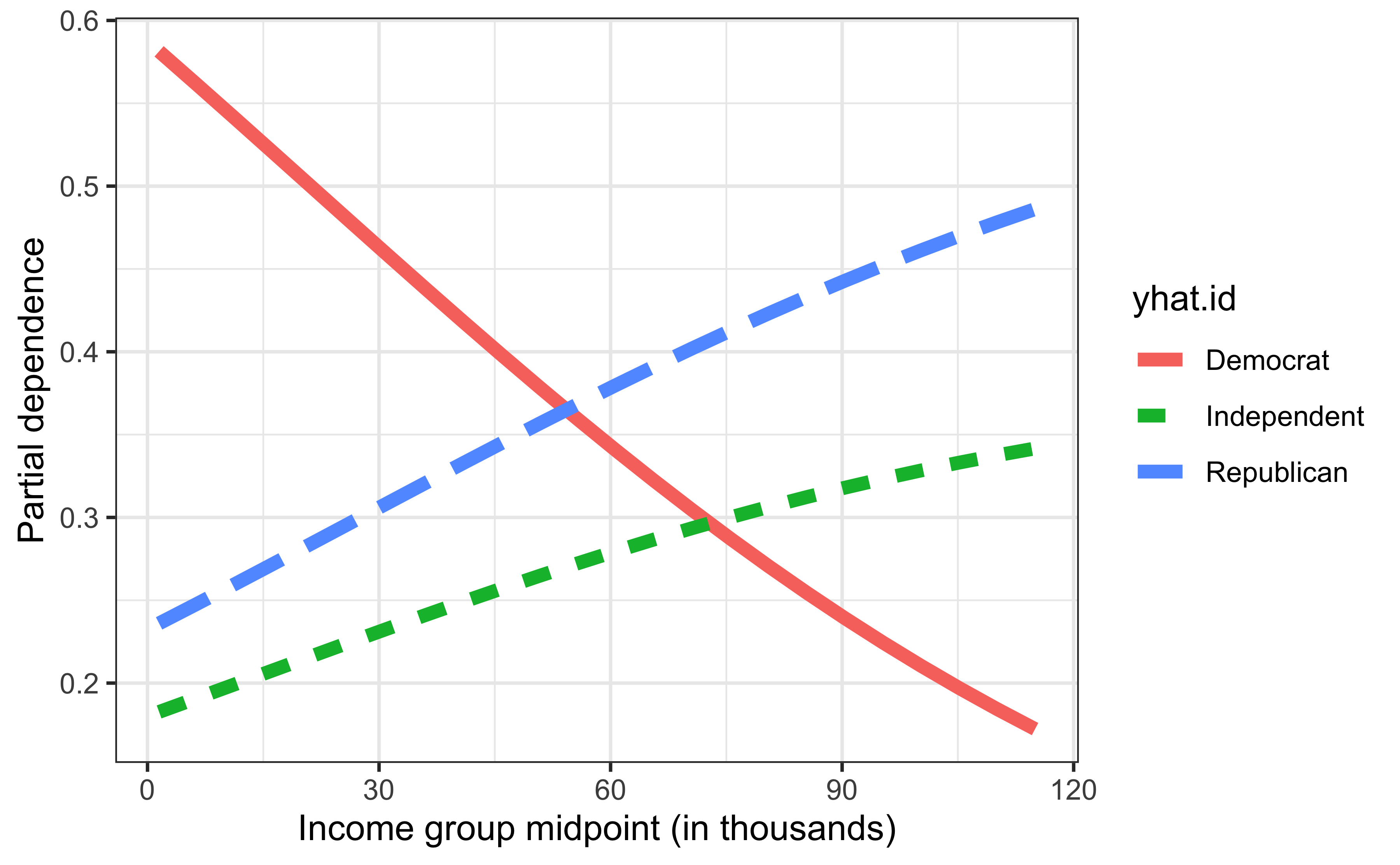

1996 National Election Study

Can perform classification, if desired…🙄

table("Predicted" = predict(mfit), "Actual" = rnes96$party)

             Actual
Predicted     Democrat Independent Republican
  Democrat         277         130        169
  Independent        4           7          5
  Republican        99         102        151

Ummm…majority of actual Republicans are classified as Democrats?!

1996 National Election Study

For kicks, try stepwise selection; since the model is based on a (multinomial) likelihood, the AIC/BIC are well-defined and the usual stepwise procedures are still valid:

(mfit2 <- MASS::stepAIC(mfit, direction = "both", scope = list("upper" = ~.^2)))

Start:  AIC=2004.33
party ~ age + education + income

                   Df    AIC
- education        12 1996.5
- age               2 2003.6
<none>                2004.3
+ age:income        2 2006.7
+ age:education    12 2009.3
+ education:income 12 2013.2
- income            2 2045.9

Step:  AIC=1996.54
party ~ age + income

             Df    AIC
- age         2 1993.4
<none>          1996.5
+ age:income  2 1998.8
+ education  12 2004.3
- income      2 2048.8

Step:  AIC=1993.42
party ~ income

            Df    AIC
<none>         1993.4
+ age        2 1996.5
+ education 12 2003.6
- income     2 2045.3

Call:
multinom(formula = party ~ income, data = rnes96, trace = FALSE)

Coefficients:
            (Intercept)     income
Independent  -1.1749331 0.01608683
Republican   -0.9503591 0.01766457

Residual Deviance: 1985.424 
AIC: 1993.424 

1996 National Election Study

For comparison, fit a (default) random forest:

set.seed(2008)  # for reproducibility
(rfo <- randomForest::randomForest(party ~ ., data = rnes96, ntree = 1000))

Call:
 randomForest(formula = party ~ ., data = rnes96, ntree = 1000) 
               Type of random forest: classification
                     Number of trees: 1000
No. of variables tried at each split: 1

        OOB estimate of  error rate: 55.72%
Confusion matrix:
            Democrat Independent Republican class.error
Democrat         248          41         91   0.3473684
Independent      129          27         83   0.8870293
Republican       156          26        143   0.5600000

1996 National Election Study

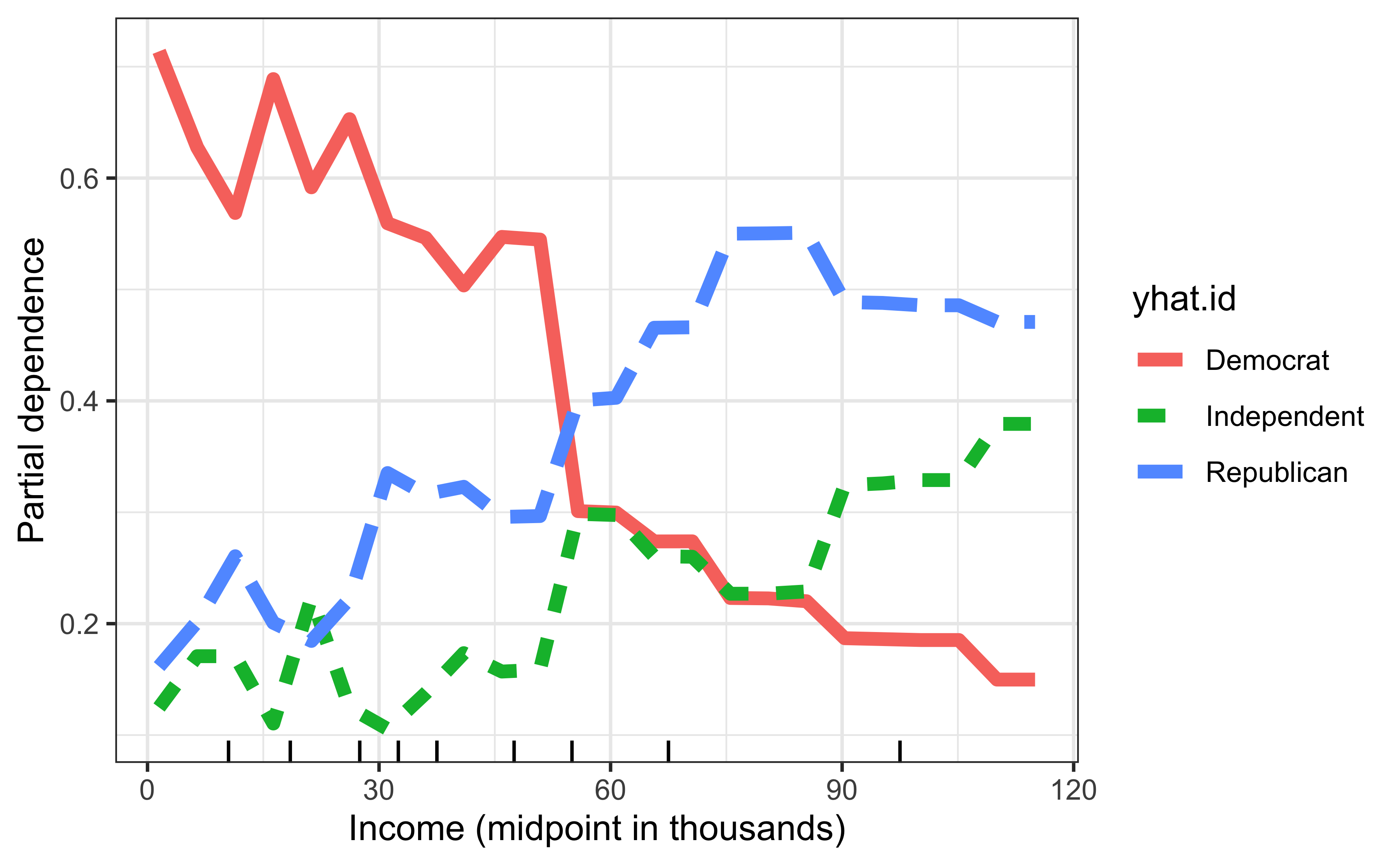
Random forest results for comparison:

# Construct the same PD plot as before, but using the RF model
pd <- partial(rfo, pred.var = "income", pred.fun = function(object, newdata) {
  colMeans(predict(object, newdata = newdata, type = "prob"))
})
ggplot(pd, aes(x = income, y = yhat, linetype = yhat.id, color = yhat.id)) +
  geom_line(size = 2) +
  xlab("Income (midpoint in thousands)") +
  ylab("Partial dependence") +
  geom_rug(data = data.frame("income" = quantile(rnes96$income, prob = 1:9/10)), aes(x = income), inherit.aes = FALSE)

Regression for Ordinal Outcomes

Ordinal outcomes

• Technically, party identification (party) is ordinal variable: Democrat < Independent < Republican

• With an ordered response (e.g., Likert scale), it’s often easier to work with the cumulative probabilities \(p_j^\le = \mathrm{P}\left(Y \le j\right)\)

• Note that if the \(J\) response categories have order \(1 < 2 < \cdots < J\), then \(p_J^\le = \mathrm{P}\left(Y \le J\right) = 1\)

• Suppose \(Z\) is some unobserved (i.e., latent) response but we only observe a discretized version of the form \(Y = j\) if \(\alpha_{j-1} < Z < \alpha_j\)

Ordinal outcomes

• If \(Z - \boldsymbol{x}^\top\boldsymbol{\beta}\) has distribution \(F\), then \[ \mathrm{P}\left(Y \le j\right) = \mathrm{P}\left(Z \le \alpha_j\right) = F\left(\alpha_j - \boldsymbol{x}^\top\boldsymbol{\beta}\right) \]

• If, for example, \(F\) is a standard logistic distribution, then \[ p_j^\le = \frac{\exp\left(\alpha_j - \boldsymbol{x}^\top\boldsymbol{\beta}\right)}{1 + \exp\left(\alpha_j - \boldsymbol{x}^\top\boldsymbol{\beta}\right)} \] which is a logit model for the cumulative probabilities!

• Choosing a standard normal distribution for \(F\) would lead to a probit model for the cumulative probabilities, and so on…

Proportional odds (PO) model

• Let \(p_j^\top = \mathrm{P}\left(Y \le j|\boldsymbol{x}\right)\)

• The standard PO model, which uses a logit link, is \[ \log\left(\frac{p_j^\le}{1-p_j^\le}\right) = \alpha_j - \boldsymbol{x}^\top\boldsymbol{\beta}, \quad j = 1, 2, \dots, J-1 \]

Proportional odds (PO) model

• PO assumption, etc…

1996 National Election Study

The simplest implementation is polr() from MASS

library(MASS)

(pofit <- polr(party ~ age + education + income, data = rnes96))

Call:
polr(formula = party ~ age + education + income, data = rnes96)

Coefficients:
         age  education.L  education.Q  education.C  education^4  education^5 
 0.005774902  0.724086814 -0.781360508  0.040168238 -0.019925492 -0.079412657 
 education^6       income 
-0.061103738  0.012738693 

Intercepts:
  Democrat|Independent Independent|Republican 
             0.6448794              1.7373541 

Residual Deviance: 1984.211 
AIC: 2004.211 

1996 National Election Study

Similar to before, we can use AIC-based stepwise procedures:

(pofit2 <- stepAIC(pofit, direction = "both"))

Start:  AIC=2004.21
party ~ age + education + income

            Df    AIC
- education  6 2002.8
<none>         2004.2
- age        1 2004.4
- income     1 2038.6

Step:  AIC=2002.83
party ~ age + income

            Df    AIC
- age        1 2001.4
<none>         2002.8
+ education  6 2004.2
- income     1 2047.2

Step:  AIC=2001.36
party ~ income

            Df    AIC
<none>         2001.4
+ age        1 2002.8
+ education  6 2004.4
- income     1 2045.3

Call:
polr(formula = party ~ income, data = rnes96)

Coefficients:
    income 
0.01311984 

Intercepts:
  Democrat|Independent Independent|Republican 
             0.2091045              1.2915566 

Residual Deviance: 1995.363 
AIC: 2001.363 

1996 National Election Study

cbind(
  "deviance" = c("PO" = deviance(pofit2), "Multi" = deviance(mfit2)),
  "nparam" = c("PO" = pofit2$edf, "Multi" = mfit2$edf)
)

      deviance nparam
PO    1995.363      3
Multi 1985.424      4

1996 National Election Study

Compare full and reduced model using LR test

anova(pofit2, pofit, test = "Chisq")

1996 National Election Study

Interpreting the coefficients:

summary(pofit2)

Call:
polr(formula = party ~ income, data = rnes96)

Coefficients:
         Value Std. Error t value
income 0.01312   0.001971   6.657

Intercepts:
                       Value   Std. Error t value
Democrat|Independent    0.2091  0.1123     1.8627
Independent|Republican  1.2916  0.1201    10.7526

Residual Deviance: 1995.363 
AIC: 2001.363 

We can say that the odds of moving from Democrat to Independent/Republican (or from Democrat/Independent to Republican) increase by a factor of \(\exp\left(0.013120\right) = 1.0132\) per unit increase in income.

Non-proportional odds (NPO) model

• We can generalize the PO model by allowing the coefficients to vary between categories (similar to the mulinomial logit model form earlier): \[ \log\left(\frac{p_j^\le}{1-p_j^\le}\right) = \alpha_j - \boldsymbol{x}^\top\boldsymbol{\beta}_j, \quad j = 1, 2, \dots, J-1 \]

• This relaxes the PO assumptions but requires more complicated software (e.g., the VGAM package)

• Careful, different packages use different default parameterizations; E.g., see Table 2 here

1996 National Election Study

PO and NPO fits to election data using VGAM:

library(VGAM)

(pofit <- vglm(party ~ income, data = rnes96,
               family = cumulative(parallel = TRUE, reverse = TRUE)))

Call:
vglm(formula = party ~ income, family = cumulative(parallel = TRUE, 
    reverse = TRUE), data = rnes96)


Coefficients:
(Intercept):1 (Intercept):2        income 
  -0.20910243   -1.29155469    0.01311978 

Degrees of Freedom: 1888 Total; 1885 Residual
Residual deviance: 1995.363 
Log-likelihood: -997.6813 

(npofit <- vglm(party ~ income, data = rnes96,
                family = cumulative(parallel = FALSE, reverse = TRUE)))

Call:
vglm(formula = party ~ income, family = cumulative(parallel = FALSE, 
    reverse = TRUE), data = rnes96)


Coefficients:
(Intercept):1 (Intercept):2      income:1      income:2 
  -0.32886794   -1.14826963    0.01618611    0.01048588 

Degrees of Freedom: 1888 Total; 1884 Residual
Residual deviance: 1987.539 
Log-likelihood: -993.7693 

Assigning scores

• When the ordinal response has a larger number of categories, it may be reasonable to assign scores (i.e., integers) to each level and then model these scores using a standard linear model

• Rule of thumb from my old advisor was 10 or more categories

Questions?