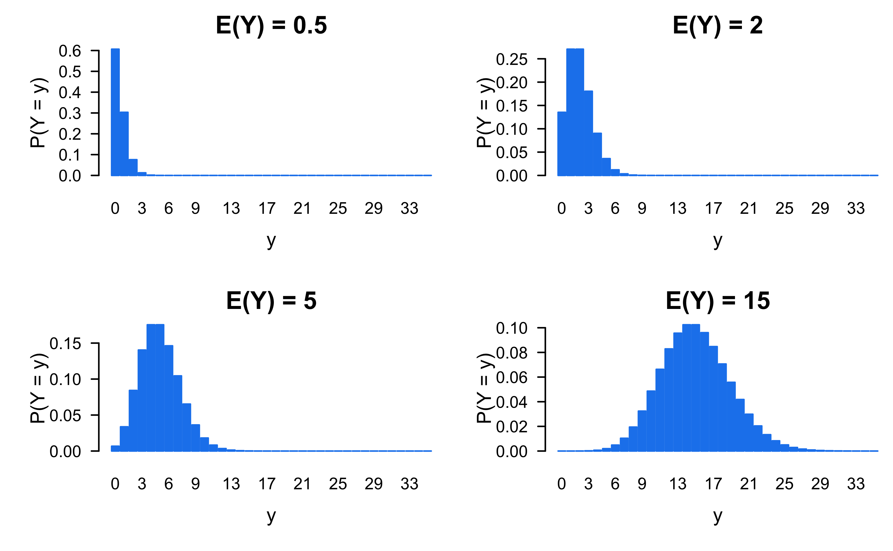
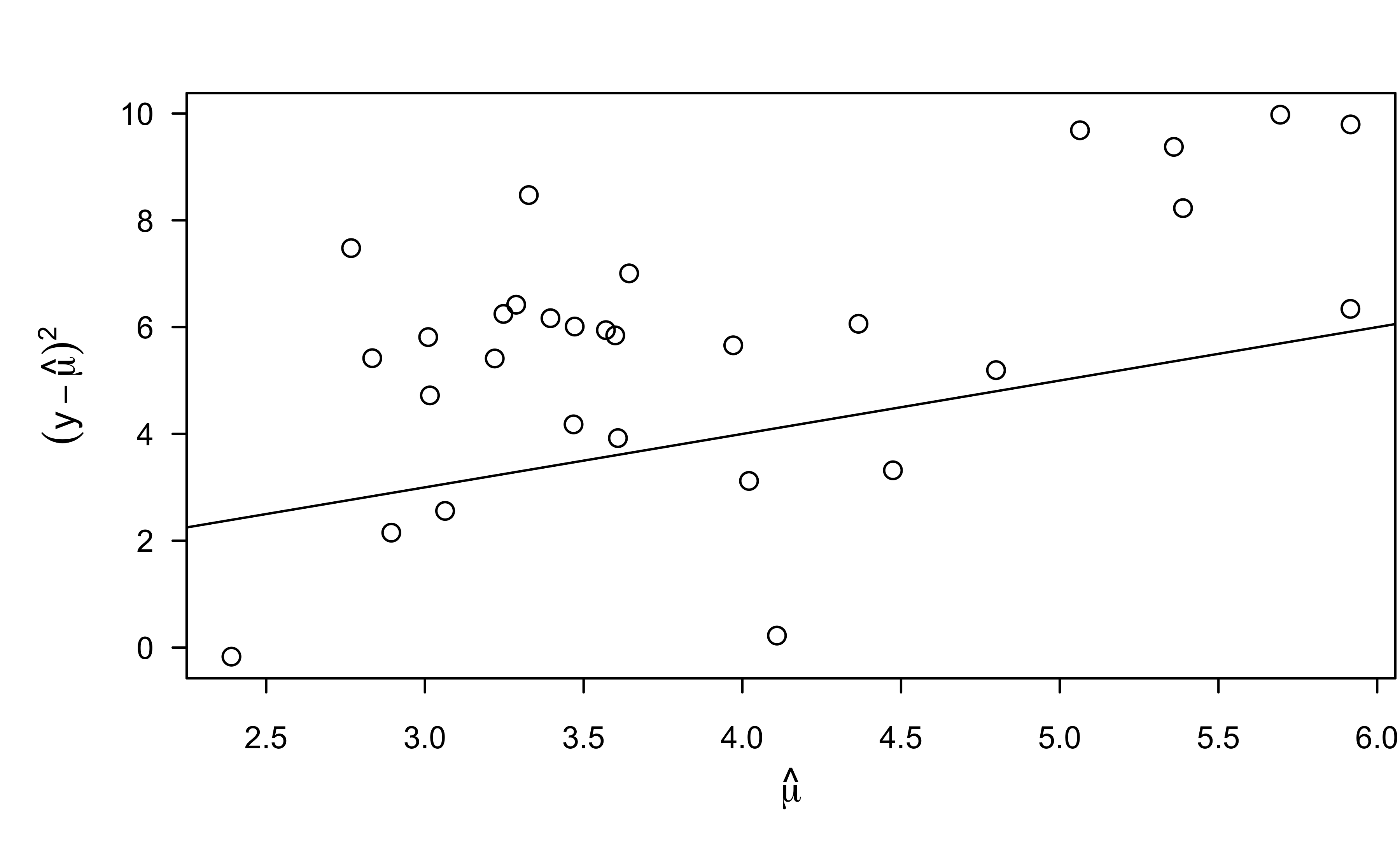
An interesting characteristic of the Poisson is that the mean and variance are equal to each other
The Poisson distribution
Show R code
# Install required package(s)pkgs <-c("faraway", "investr", "mgcv", "performance", "pscl")lib <-installed.packages()[, "Package"]install.packages(setdiff(pkgs, lib))# Y ~ Poisson(lambda = 0.5)set.seed(2004) # for reproducibilitypar(mfrow =c(2, 2))for (lambda inc(0.5, 2, 5, 15)) { y <-dpois(0:35, lambda = lambda)barplot(y, xlab ="y", ylab ="P(Y = y)", names =0:35, main =paste("E(Y) =", lambda), col ="dodgerblue2", border ="dodgerblue2", las =1)}
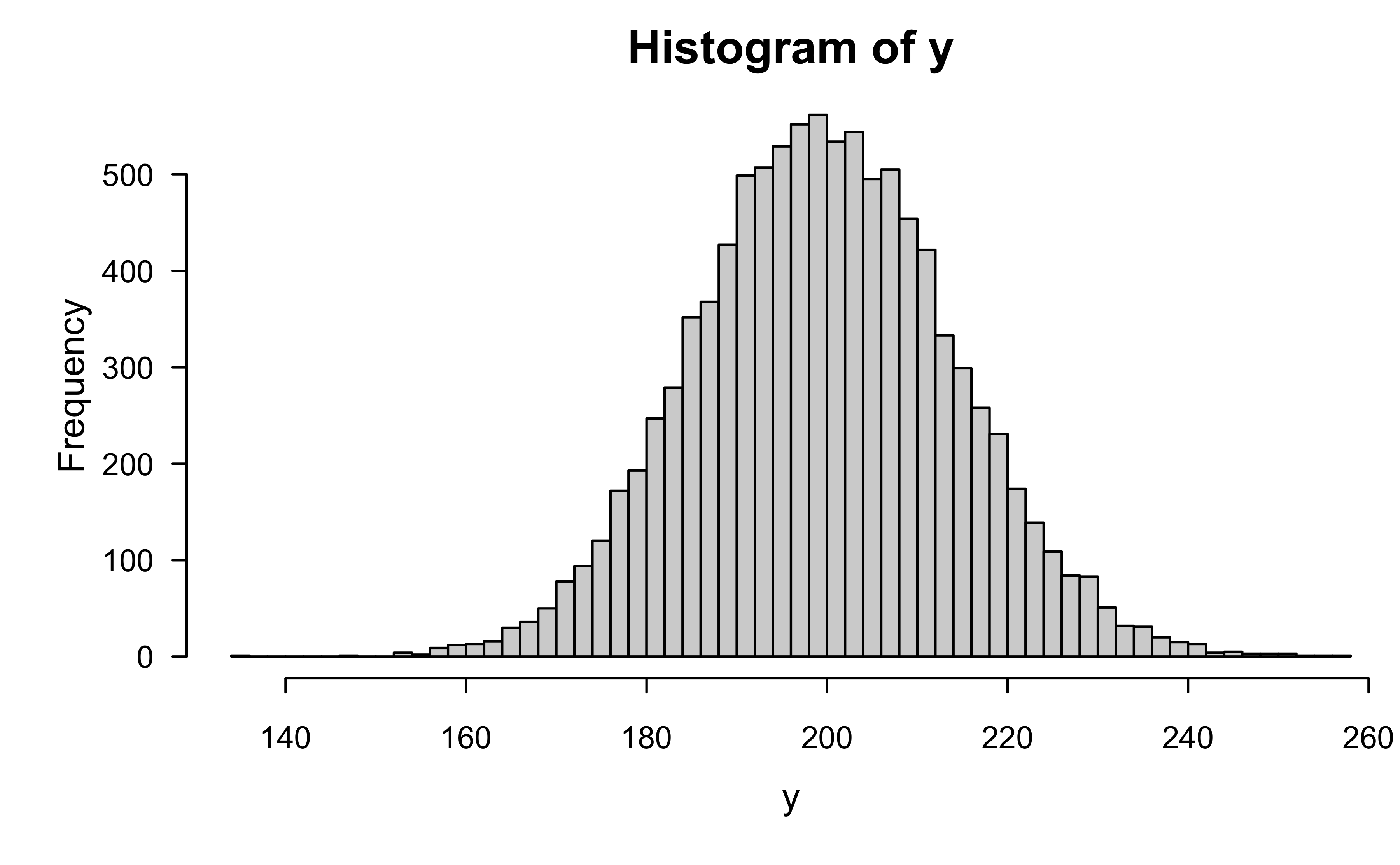
The Poisson distribution
Show R code
y <-rpois(10000, lambda =200)hist(y, br =50)
The Poisson distribution
If the count is some number out of some possible total, then the response would be more appropriately modeled as a binomial r.v.
However, for small \(p\) and large \(n\), the Poisson distribution provides a reasonable approximation to the binomial; For example, in modeling the incidence of rare forms of cancer, the number of people affected is a small proportion of the population in a given geographical area
Show R code
c("Binomial"=pbinom(5, size =8, p =0.7),"Poisson"=ppois(5, lambda =8*0.7))
 Binomial   Poisson
0.4482262 0.5118609
Show R code
c("Binomial"=pbinom(5, size =100, p =0.05),"Poisson"=ppois(5, lambda =100*0.05))
 Binomial   Poisson
0.6159991 0.6159607
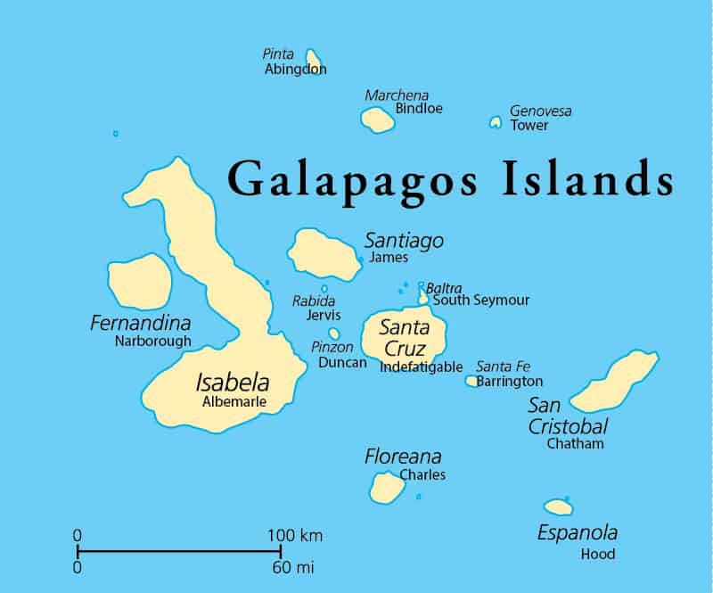
Galápagos islands data
There are 30 Galapagos islands and 7 variables in the data set. The relationship between the number of plant species (\(Y\)) and several geographic variables is of interest. The original data set contained several missing values which have been filled for convenience. See the faraway::galamiss data set for the original version.
Galápagos islands data
Galápagos islands data
We’ll remove Endemics since we won’t be using it!
Show R code
# Load the Galapagos Islands datadata(gala, package ="faraway")gala$Endemics <-NULL# Print structure of data framestr(gala)
'data.frame':   30 obs. of  6 variables:
 $ Species  : num  58 31 3 25 2 18 24 10 8 2 ...
 $ Area     : num  25.09 1.24 0.21 0.1 0.05 ...
 $ Elevation: num  346 109 114 46 77 119 93 168 71 112 ...
 $ Nearest  : num  0.6 0.6 2.8 1.9 1.9 8 6 34.1 0.4 2.6 ...
 $ Scruz    : num  0.6 26.3 58.7 47.4 1.9 ...
 $ Adjacent : num  1.84 572.33 0.78 0.18 903.82 ...
Galápagos islands data
Summary of data frame
Show R code
summary(gala)
    Species            Area             Elevation          Nearest
 Min.   :  2.00   Min.   :   0.0100   Min.   :  25.00   Min.   : 0.20
 1st Qu.: 13.00   1st Qu.:   0.2575   1st Qu.:  97.75   1st Qu.: 0.80
 Median : 42.00   Median :   2.5900   Median : 192.00   Median : 3.05
 Mean   : 85.23   Mean   : 261.7087   Mean   : 368.03   Mean   :10.06
 3rd Qu.: 96.00   3rd Qu.:  59.2375   3rd Qu.: 435.25   3rd Qu.:10.03
 Max.   :444.00   Max.   :4669.3200   Max.   :1707.00   Max.   :47.40
     Scruz           Adjacent
 Min.   :  0.00   Min.   :   0.03
 1st Qu.: 11.03   1st Qu.:   0.52
 Median : 46.65   Median :   2.59
 Mean   : 56.98   Mean   : 261.10
 3rd Qu.: 81.08   3rd Qu.:  59.24
 Max.   :290.20   Max.   :4669.32
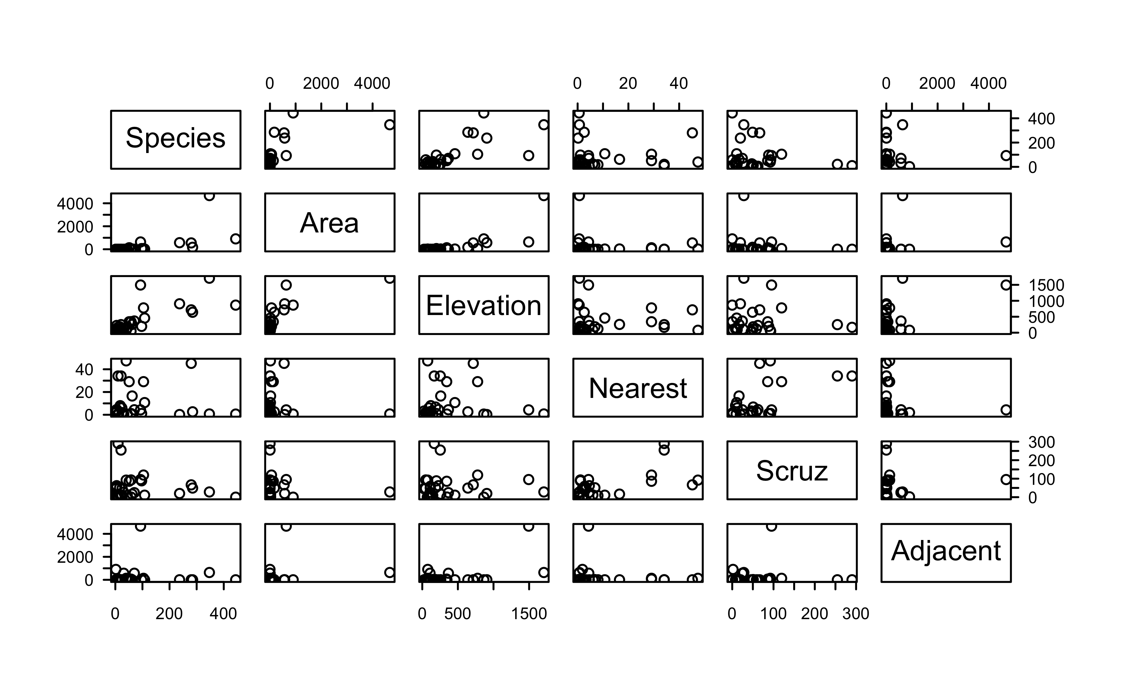
Galápagos islands data
Show R code
pairs(gala)
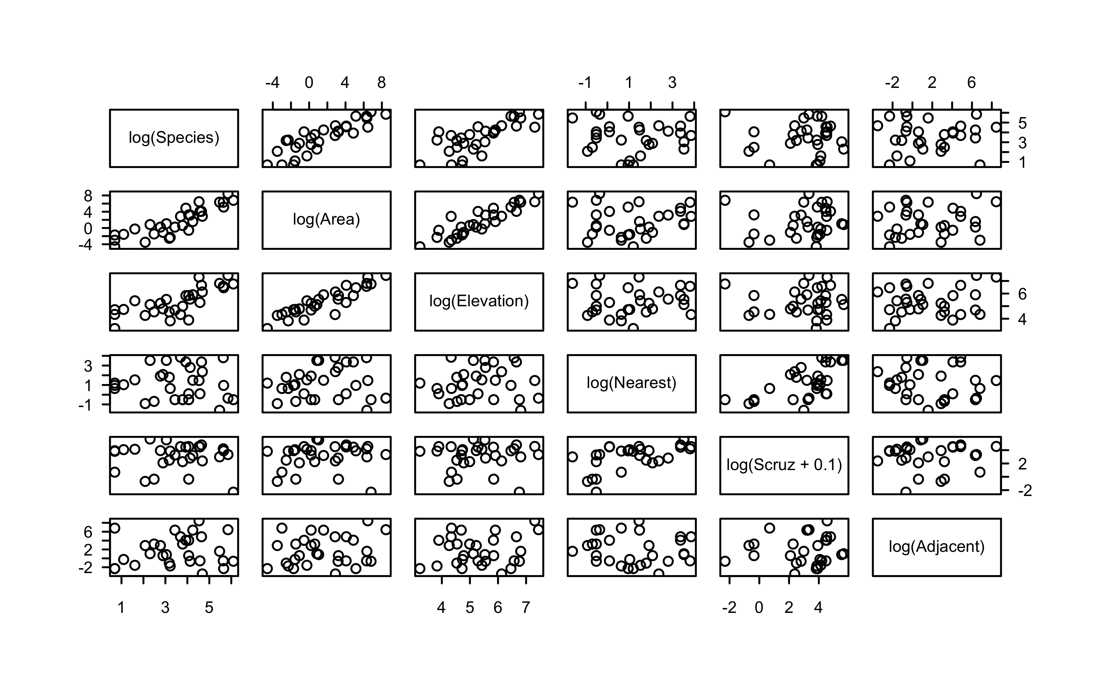
Galápagos islands data
Show R code
pairs(~log(Species) +log(Area) +log(Elevation) +log(Nearest) +log(Scruz +0.1) +log(Adjacent), data = gala)
Call:
lm(formula = log(Species) ~ log(Area) + log(Elevation) + log(Nearest) +
    I(log(Scruz + 0.1)) + log(Adjacent), data = gala)

Residuals:
    Min      1Q  Median      3Q     Max
-1.4563 -0.5192 -0.1059  0.4632  1.3351

Coefficients:
                    Estimate Std. Error t value Pr(>|t|)
(Intercept)          5.10569    1.64880   3.097  0.00493 **
log(Area)            0.50350    0.09942   5.064 3.53e-05 ***
log(Elevation)      -0.37384    0.32242  -1.159  0.25767
log(Nearest)        -0.06564    0.11475  -0.572  0.57262
I(log(Scruz + 0.1)) -0.08255    0.09517  -0.867  0.39433
log(Adjacent)       -0.02488    0.04596  -0.541  0.59327
---
Signif. codes:  0 '***' 0.001 '**' 0.01 '*' 0.05 '.' 0.1 ' ' 1

Residual standard error: 0.7877 on 24 degrees of freedom
Multiple R-squared:  0.7899,    Adjusted R-squared:  0.7461
F-statistic: 18.05 on 5 and 24 DF,  p-value: 1.941e-07
Galápagos islands data
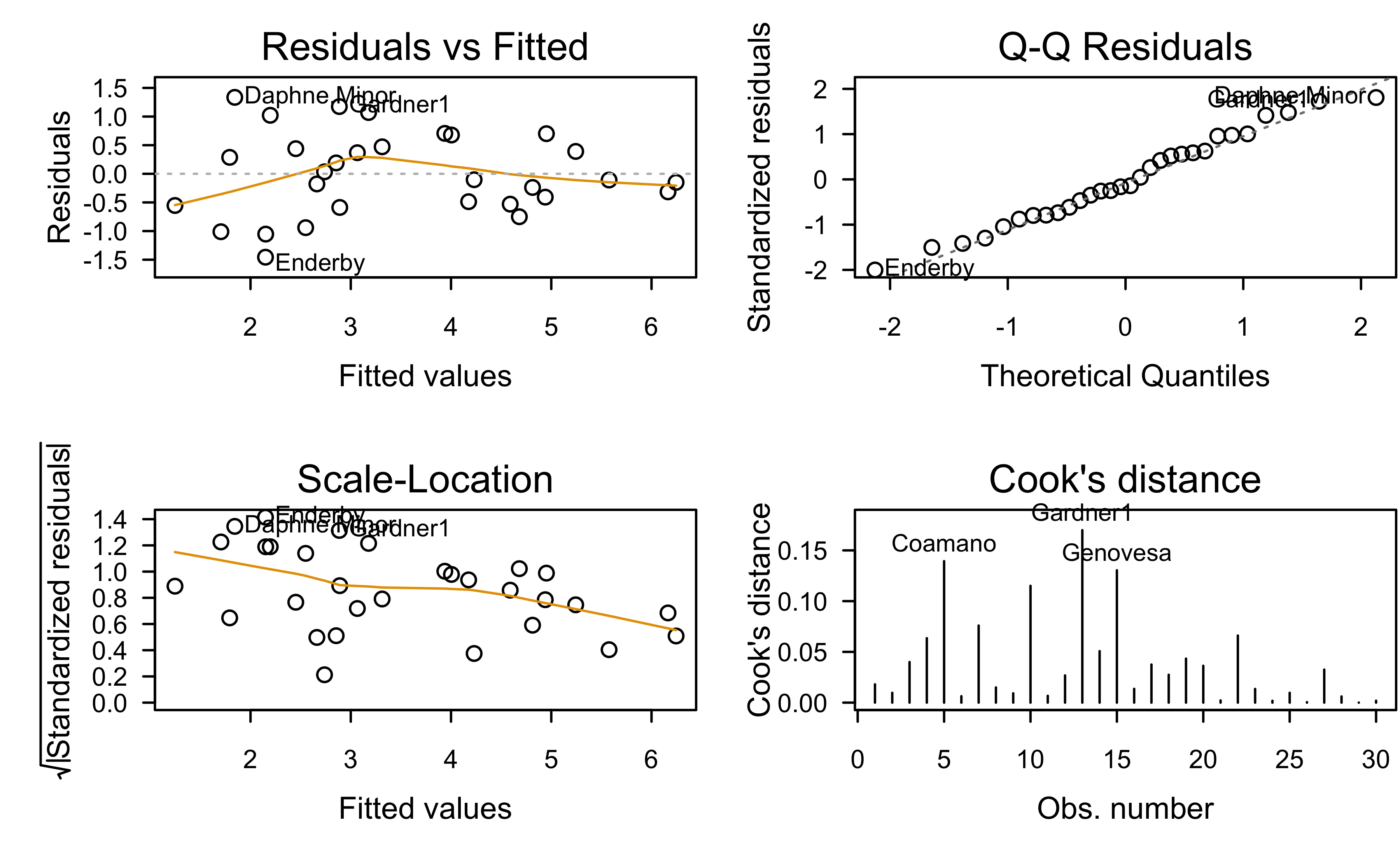
Residual analysis
Show R code
par(mfrow =c(2, 2))plot(gala.ols, which =1:4)
Poisson regression
Need a way to link the mean response \(\mathrm{E}\left(Y\right) = \mu \in \left(0, \infty\right)\) to the linear predictor \(\eta = \boldsymbol{x}^\top\boldsymbol{p}\)
In Poisson we regression, we default to \[
\log\left(\mu\right) = \boldsymbol{x}^\top\boldsymbol{p}
\]
Maximum likelihood estimation provides a convenient estimate of \(\boldsymbol{\beta}\)
Galápagos islands data
Try a Poisson regression
Show R code
summary(gala.poi <-glm(Species ~ ., data = gala, family = poisson))
Call:
glm(formula = Species ~ ., family = poisson, data = gala)

Coefficients:
              Estimate Std. Error z value Pr(>|z|)
(Intercept)  3.155e+00  5.175e-02  60.963  < 2e-16 ***
Area        -5.799e-04  2.627e-05 -22.074  < 2e-16 ***
Elevation    3.541e-03  8.741e-05  40.507  < 2e-16 ***
Nearest      8.826e-03  1.821e-03   4.846 1.26e-06 ***
Scruz       -5.709e-03  6.256e-04  -9.126  < 2e-16 ***
Adjacent    -6.630e-04  2.933e-05 -22.608  < 2e-16 ***
---
Signif. codes:  0 '***' 0.001 '**' 0.01 '*' 0.05 '.' 0.1 ' ' 1

(Dispersion parameter for poisson family taken to be 1)

    Null deviance: 3510.73  on 29  degrees of freedom
Residual deviance:  716.85  on 24  degrees of freedom
AIC: 889.68

Number of Fisher Scoring iterations: 5
# Overdispersion test

       dispersion ratio =  31.749
  Pearson's Chi-Squared = 761.979
                p-value = < 0.001
Overdispersion detected.
Galápagos islands data
Similar to before, can use quasipoisson() family to correct fo overdispersion:
Show R code
gala.quasipoi <-glm(Species ~ ., family =quasipoisson(link ="log"), data = gala)summary(gala.quasipoi)
Call:
glm(formula = Species ~ ., family = quasipoisson(link = "log"),
    data = gala)

Coefficients:
              Estimate Std. Error t value Pr(>|t|)
(Intercept)  3.1548079  0.2915901  10.819 1.03e-10 ***
Area        -0.0005799  0.0001480  -3.918 0.000649 ***
Elevation    0.0035406  0.0004925   7.189 1.98e-07 ***
Nearest      0.0088256  0.0102622   0.860 0.398292
Scruz       -0.0057094  0.0035251  -1.620 0.118380
Adjacent    -0.0006630  0.0001653  -4.012 0.000511 ***
---
Signif. codes:  0 '***' 0.001 '**' 0.01 '*' 0.05 '.' 0.1 ' ' 1

(Dispersion parameter for quasipoisson family taken to be 31.74921)

    Null deviance: 3510.73  on 29  degrees of freedom
Residual deviance:  716.85  on 24  degrees of freedom
AIC: NA

Number of Fisher Scoring iterations: 5
Rates and offsets
The number of observed events may depend on a size variable that determines the number of opportunities for the events to occur
For example, the number of burglaries reported in different cities
In other cases, the size variable may be time
For example, the number of customers served by a sales worker (must take account of the differing amounts of time worked)
Rates and offsets
An experiment was conducted to determine the effect of gamma radiation on the numbers of chromosomal abnormalities (ca) observed. The number (cells), in hundreds of cells exposed in each run, differs. The dose amount (doseamt) and the rate (doserate) at which the dose is applied are the predictors of interest. The hypothesized model is as follows:
dicentric <- faraway::dicentricdicentric$dosef <-factor(dicentric$doseamt)fit <-glm(ca ~offset(log(cells)) +log(doserate)*dosef, family = poisson, data = dicentric)summary(fit)
Call:
glm(formula = ca ~ offset(log(cells)) + log(doserate) * dosef,
    family = poisson, data = dicentric)

Coefficients:
                       Estimate Std. Error z value Pr(>|z|)
(Intercept)            -2.74671    0.03426 -80.165  < 2e-16 ***
log(doserate)           0.07178    0.03518   2.041 0.041299 *
dosef2.5                1.62542    0.04946  32.863  < 2e-16 ***
dosef5                  2.76109    0.04349  63.491  < 2e-16 ***
log(doserate):dosef2.5  0.16122    0.04830   3.338 0.000844 ***
log(doserate):dosef5    0.19350    0.04243   4.561  5.1e-06 ***
---
Signif. codes:  0 '***' 0.001 '**' 0.01 '*' 0.05 '.' 0.1 ' ' 1

(Dispersion parameter for poisson family taken to be 1)

    Null deviance: 4753.00  on 26  degrees of freedom
Residual deviance:   21.75  on 21  degrees of freedom
AIC: 209.16

Number of Fisher Scoring iterations: 4
zero-inflated outcomes
The state wildlife biologists want to model how many fish are being caught by fishermen at a state park. Visitors are asked how long they stayed, how many people were in the group, were there children in the group, and how many fish were caught. Some visitors do not fish, but there is no data on whether a person fished or not. Some visitors who did fish did not catch any fish so there are excess zeros in the data because of the people that did not fish.
Zero-inflated outcomes
Our sample consists of We have data on N=250 groups that went to a park. Each group was questioned about how many fish they caught (count), how many children were in the group (child), how many people were in the group (persons), and whether or not they brought a camper to the park (camper).
The data can be read in as follows:
fish <-read.csv("https://stats.idre.ucla.edu/stat/data/fish.csv")
Zero-inflated outcomes
# Retain only variables of interest and print summaryfish <- fish[, c("count", "child", "persons", "camper")]summary(fish)
     count             child          persons          camper
 Min.   :  0.000   Min.   :0.000   Min.   :1.000   Min.   :0.000
 1st Qu.:  0.000   1st Qu.:0.000   1st Qu.:2.000   1st Qu.:0.000
 Median :  0.000   Median :0.000   Median :2.000   Median :1.000
 Mean   :  3.296   Mean   :0.684   Mean   :2.528   Mean   :0.588
 3rd Qu.:  2.000   3rd Qu.:1.000   3rd Qu.:4.000   3rd Qu.:1.000
 Max.   :149.000   Max.   :3.000   Max.   :4.000   Max.   :1.000
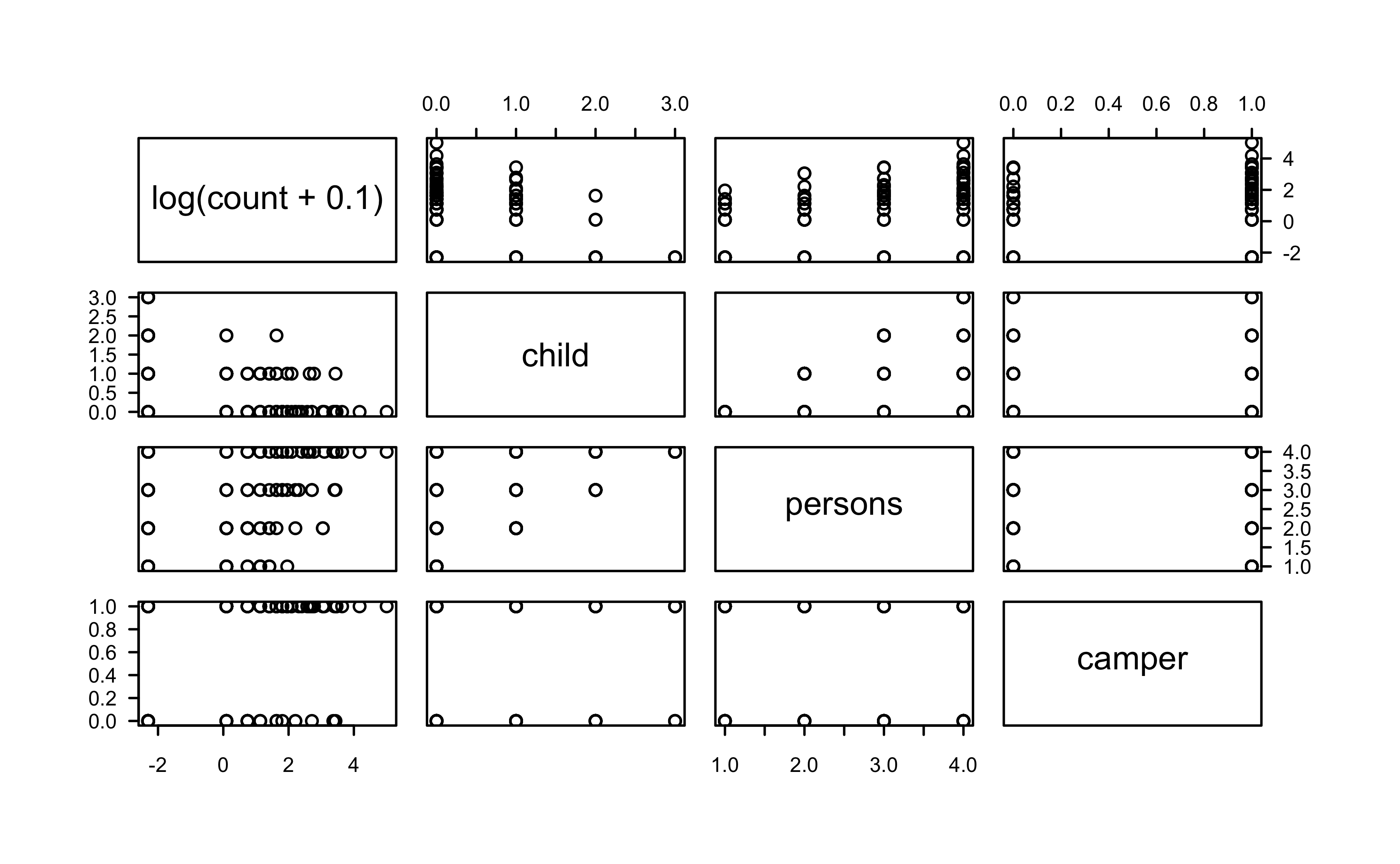
Zero-inflated outcomes
Show R code
pairs(log(count +0.1) ~ ., data = fish)
Zero-inflated outcomes
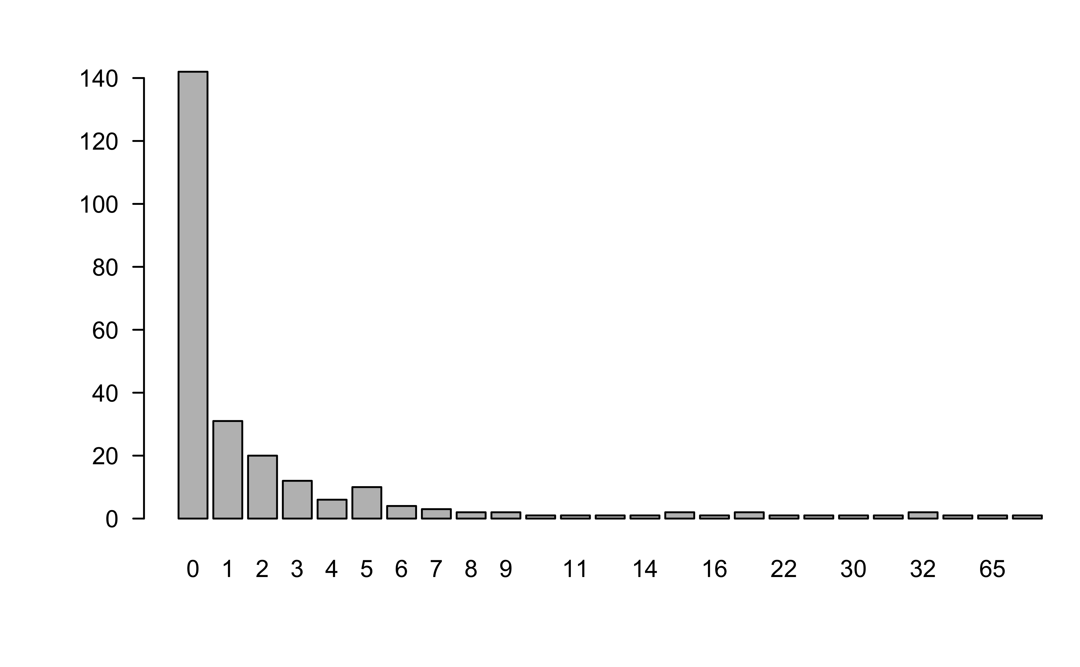
Too many zeros?
Show R code
barplot(table(fish$count))
Zero-inflated outcomes
fish.poi <-glm(count ~ ., data = fish, family = poisson)summary(fish.poi)
Call:
glm(formula = count ~ ., family = poisson, data = fish)

Coefficients:
            Estimate Std. Error z value Pr(>|z|)
(Intercept) -1.98183    0.15226  -13.02   <2e-16 ***
child       -1.68996    0.08099  -20.87   <2e-16 ***
persons      1.09126    0.03926   27.80   <2e-16 ***
camper       0.93094    0.08909   10.45   <2e-16 ***
---
Signif. codes:  0 '***' 0.001 '**' 0.01 '*' 0.05 '.' 0.1 ' ' 1

(Dispersion parameter for poisson family taken to be 1)

    Null deviance: 2958.4  on 249  degrees of freedom
Residual deviance: 1337.1  on 246  degrees of freedom
AIC: 1682.1

Number of Fisher Scoring iterations: 6
Model is underfitting zeros (probable zero-inflation).
The hurdle model
In addition to predicting the number of fish caught, there is interest in predicting the existence of excess zeros (i.e., the zeroes that were not simply a result of bad luck or lack of fishing skill). In particular, we’d like to estimate the effect of party size on catching zero fish.
We can accomplish this in several ways, but popular choices include:
The zero-inflated Poisson (or negative binomial) model
The hurdle model
The hurdle model
In this example, we’ll use a simple hurdle model, which essentially fits two separate models:
\(\mathrm{P}\left(Y = 0\right)\) via a logistic regression
\(\mathrm{P}\left(Y = j\right)\), \(j = 1, 2, \dots\) via a truncated Poisson regression
The hurdle model
You can fit hurdle models using the hurdle() function from package pscl: