Computing and visualizing functional residuals with the funres package • funres

library(funres)

Currently supported models

Model type	Family	Package	Function
GLM	Binomial	stats	`glm()`
GLM	Poisson	stats	`glm()`
GLM	Quasi-Poisson	stats	`glm()`
GAM	Binomial	mgcv	`gam()`
GAM	Poisson	mgcv	`gam()`
GAM	Quasi-Poisson	mgcv	`gam()`
Ordinal	NA	VGAM	`vgam()` and `vgam()`

Logistic regression

We’ll start by generating data from a quadratic logistic regression (LR) model:

# Generate data from a logistic regression model with quadratic form
set.seed(1217)
n <- 1000
x <- rnorm(n)
# x[1] <- 10  # add an outlier
z <- 1 - 2*x + 3*x^2 + rlogis(n)
y <- ifelse(z > 0, 1, 0)

# Fit a couple of LR models
fit.bad <- glm(y ~ x, family = binomial)  # wrong
fit.good <- glm(y ~ x + I(x^2), family = binomial)  # right
#> Warning: glm.fit: fitted probabilities numerically 0 or 1 occurred

Functional residuals

fres.bad <- fresiduals(fit.bad)
fres.good <- fresiduals(fit.good)
par(mfrow = c(1, 2), las = 1)
plot(fres.bad[[1]], xlab = "t", ylab = "F(t)")
plot(fres.good[[1]], xlab = "t", ylab = "F(t)")  # plot FRs for first observation

Does plotting them all tell us anything interesting?

plot(fres.bad[[1]], xlab = "t", ylab = "F(t)", las = 1, type = "n")
tt <- 0:100/100
for (i in seq_along(fres.bad)) {
  lines(tt, fres.bad[[i]](tt), col = adjustcolor(1, alpha.f = 0.05))
}

Surrogate and probability-scale residuals

sr.bad <- fresiduals(fit.bad, type = "surrogate")
sr.good <- fresiduals(fit.good, type = "surrogate")
par(mfrow = c(1, 2))
col <- adjustcolor(1, alpha.f = 0.2)
plot(x, y = sr.bad, col = col, las = 1, ylab = "Surrogate residual")
lines(lowess(x, y = sr.bad), lwd = 2, col = "red2")
plot(x, y = sr.good, col = col, las = 1, ylab = "Surrogate residual")
lines(lowess(x, y = sr.good), lwd = 2, col = "red2")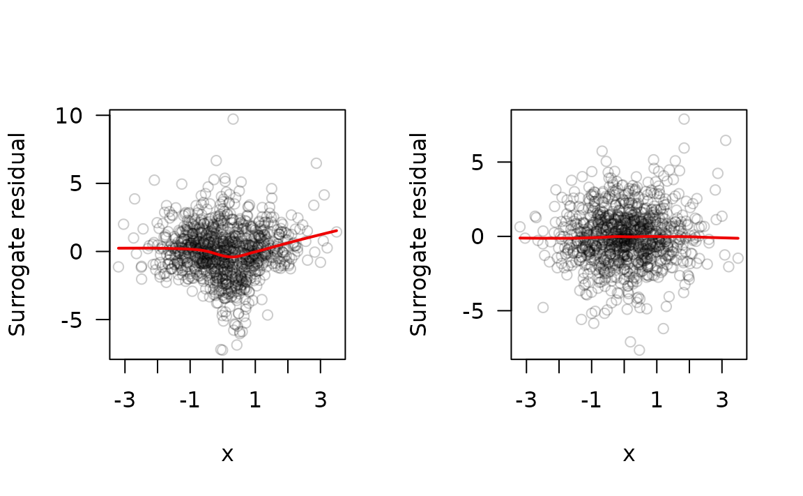

# Probability-scale residuals
ps.bad <- fresiduals(fit.bad, type = "probscale")
ps.good <- fresiduals(fit.good, type = "probscale")
par(mfrow = c(1, 2))
plot(x, y = ps.bad, col = col, las = 1, ylab = "Surrogate residual")
lines(lowess(x, y = sr.bad), lwd = 2, col = "red2")
plot(x, y = ps.good, col = col, las = 1, ylab = "Surrogate residual")
lines(lowess(x, y = sr.good), lwd = 2, col = "red2")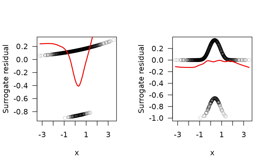

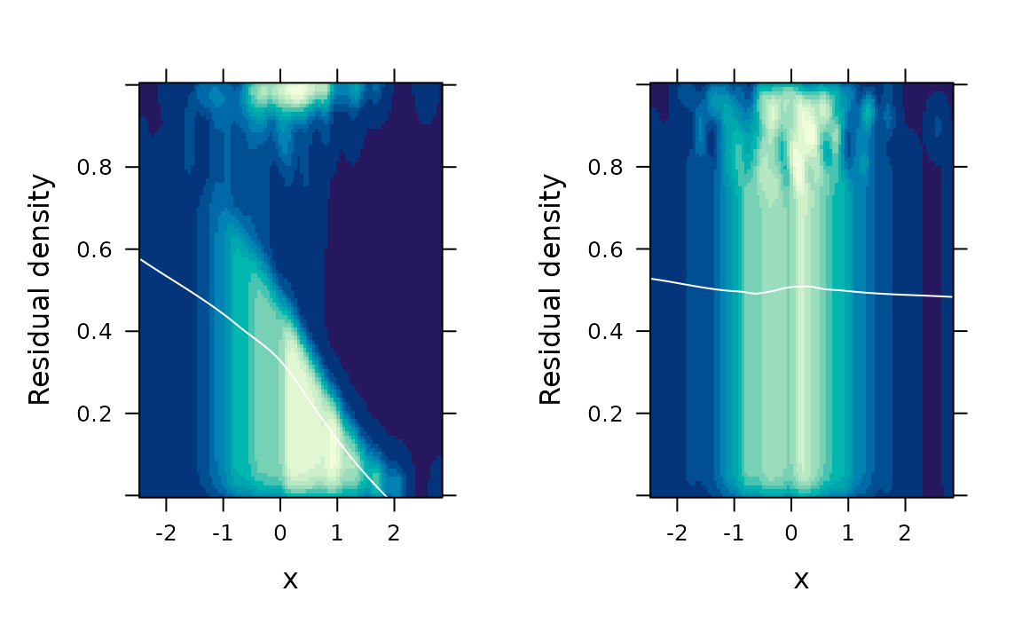
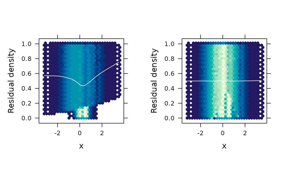
Functional residual density (FRED) plots

The FRED plots in R are based on the Trellis framework (e.g., lattice), which rely on grid graphics. The gridExtra::grid.arrange() function is the most convenient approach to arranging several plots here. These graphs are quicker to produce compared to ggplot2.

# Two-dimensional kernel density estimation
gridExtra::grid.arrange(
  fredplot(fit.bad, x = x),
  fredplot(fit.good, x = x),
  nrow = 1
)


# Hexagonal binning
gridExtra::grid.arrange(
  fredplot(fit.bad, x = x, type = "hex", aspect = 1),
  fredplot(fit.good, x = x, type = "hex", aspect = 1),
  nrow = 1
)

Function-function plots

palette("Okabe-Ito")
par(mfrow = c(1, 2))
ffplot(fit.bad, n = 500, type = "l")
ffplot(fit.good, n = 500, type = "l")

palette("default")

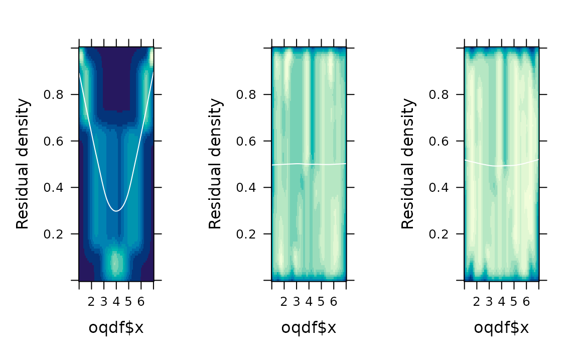
Ordinal model example with VGAM package

library(VGAM)
#> Loading required package: stats4
#> Loading required package: splines


# Helper functions to simulate quadratic ordinal response data
ordinalize <- function(z, threshold) {
  sapply(z, FUN = function(x) {
    ordinal.value <- 1
    index <- 1
    while(index <= length(threshold) && x > threshold[index]) {
      ordinal.value <- ordinal.value + 1
      index <- index + 1
    }
    ordinal.value
  })
}
simoqd <- function(n = 2000) {
  threshold <- c(0, 4, 8)
  x <- runif(n, min = 1, max = 7)
  z <- 16 - 8 * x + 1 * x ^ 2 + rnorm(n)  # rlnorm(n)
  y <- sapply(z, FUN = function(zz) {
    ordinal.value <- 1
    index <- 1
    while(index <= length(threshold) && zz > threshold[index]) {
      ordinal.value <- ordinal.value + 1
      index <- index + 1
    }
    ordinal.value
  })
  data.frame("y" = as.ordered(y), "x" = x)
}

# Simulate data
set.seed(977)
oqdf <- simoqd(n = 2000)

# Fit models to simulated ordinal quadratice response data
fit1 <- vglm(y ~ x, data = oqdf, family = acat(reverse = TRUE, parallel = TRUE))
fit2 <- vglm(y ~ poly(x, degree = 2), data = oqdf, family = acat(reverse = TRUE, parallel = TRUE))
#> Warning in checkwz(wz, M = M, trace = trace, wzepsilon = control$wzepsilon): 1
#> diagonal elements of the working weights variable 'wz' have been replaced by
#> 1.819e-12
#> Warning in checkwz(wz, M = M, trace = trace, wzepsilon = control$wzepsilon): 6
#> diagonal elements of the working weights variable 'wz' have been replaced by
#> 1.819e-12
#> Warning in checkwz(wz, M = M, trace = trace, wzepsilon = control$wzepsilon): 6
#> diagonal elements of the working weights variable 'wz' have been replaced by
#> 1.819e-12
fit3 <- vgam(y ~ s(x), data = oqdf, family = acat(reverse = TRUE, parallel = TRUE))
#> Warning in vgam.fit(x = x, y = y, w = w, mf = mf, Xm2 = Xm2, Ym2 = Ym2, :
#> convergence not obtained in 30 IRLS iterations

# Residual plots
gridExtra::grid.arrange(
  fredplot(fit1, x = oqdf$x),  # linear term (wrong)
  fredplot(fit2, x = oqdf$x),  # quadratic term
  fredplot(fit3, x = oqdf$x),  # smooth term
  nrow = 1
)

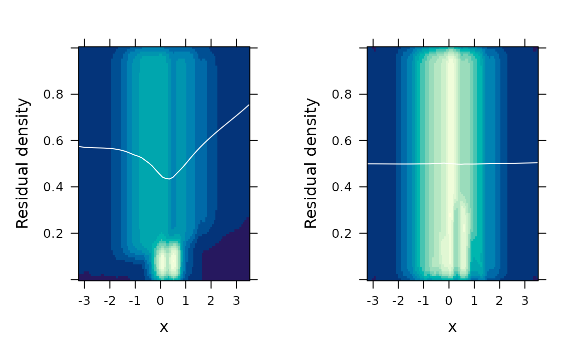
Zero-inflated Poisson (ZIP) model

# library(VGAM)
# library(pscl)

# Simulate ZIP data
set.seed(3)
x <- rnorm(1000, 0, 0.8)
lp <- 1 + 1 * x  # linear predictor
lambda <- exp(lp)
p0 <- exp(1 + 0.2 * x) / (exp( 1 + 0.2 * x) + 1)
y <- VGAM::rzipois(1000, lambda = lambda, pstr0 = p0)
df <- cbind.data.frame(x, y)

fit1 <- glm(y ~ x, family = poisson, data = df)
fit2 <- pscl::zeroinfl(y ~ x, data = df)

gridExtra::grid.arrange(
  fredplot(fit1, x = x),
  fredplot(fit2, x = x),
  ncol = 2
)