Introduction to surrogate residuals in R

Brad Boehmke & Brandon Greenwell

2026-07-07

Introduction

Categorical outcomes are encountered frequently in practice across different fields. For example, in medical studies, the outcome of interest is often binary (e.g., presence or absence of a particular disease after applying a treatment). In other studies, the outcome may be an ordinal variable; that is, a categorical outcome having a natural ordering. For instance, in an opinion poll, the response may be satisfaction, with categories low, medium, and high. In this case, the response is ordered: low $<$ medium $<$ high.

Logistic and probit regression are popular choices for modelling a binary outcome. Although this paper focuses on models for ordinal responses, the surrogate approach to constructing residuals actually applies to a wide class of general models of the form

$$Y \sim F_a\left(y; \boldsymbol{X}, \boldsymbol{\beta}\right),$$

where $F_a\left(\cdot\right)$ is a discrete cumulative distribution function, $\boldsymbol{X}$, is an $n \times p$ model matrix, and $\boldsymbol{\beta}$ is a $p \times 1$ vector of unknown regression coefficients. This includes binary regression as a special case. For example, the probit model has

$$Y \sim Bernoulli\left[\Phi\left(\boldsymbol{X}^\top\boldsymbol{\beta}\right)\right],$$

where $\Phi\left(\cdot\right)$ is the cumulative distribution function for the standard normal distribution.

The cumulative link model is a natural choice for modelling a binary or ordinal outcome. Consider an ordinal categorical outcome $Y$ with ordered categories $1 < 2 < \dots < J$. In a cumulative link model, the cumulative probabilities are linked to the predictors according to

$$G^{-1}\left(\Pr\left\{Y \le j\right\}\right) = \alpha_j + f\left(\boldsymbol{X}, \boldsymbol{\beta}\right), \tag{1}$$

where $G\left(\cdot\right)$ is a continuous cumulative distribution function, $\alpha_j$ are the category-specific intercepts, $\boldsymbol{X}$ is a matrix of covariates, and $\boldsymbol{\beta}$ is a vector of fixed regression coefficients. The intercept parameters satisfy $-\infty = \alpha_0 < \alpha_1 < \dots < \alpha_{J-1} < \alpha_J = \infty$. We should point out that some authors (and software) use the alternate formulation

$$G^{-1}\left(\Pr\left\{Y \ge j\right\}\right) = \alpha_j^\star + f\left(\boldsymbol{X}, \boldsymbol{\beta}^\star\right). \tag{2}$$

This formulation provides coefficients that are consistent with the ordinary logistic regression model. The estimated coefficients from model (2) will have the opposite sign as those in model (1); see, for example, Agresti (2010).

Another way to interpret the cumulative link model is through a latent continuous random variable $Z = -f\left(\boldsymbol{X}, \boldsymbol{\beta}\right) + \epsilon$, where $\epsilon$ is a continuous random variable with location parameter $0$, scale parameter $1$, and cumulative distribution function $G\left(\cdot\right)$. We then construct an ordered factor according to the rule

$$y = j \quad if \quad \alpha_{j - 1} < z \le \alpha_j.$$

For $\epsilon \sim N\left(0, 1\right)$, this leads to the usual probit model for ordinal responses,

$$\Pr\left\{Y \le j\right\} = \Pr\left\{Z \le \alpha_j\right\} = \Pr\left\{-f\left(\boldsymbol{X}, \boldsymbol{\beta}\right) + \epsilon \le \alpha_j\right\} = \Phi\left(\alpha_j + f\left(\boldsymbol{X}, \boldsymbol{\beta}\right)\right).$$

Common choices for the link function $G^{-1}\left(\cdot\right)$ and the implied (standard) distribution for $\epsilon$ are described in Table 1.

Link	Distribution of $\epsilon$	$G\left(y\right)$	$G^{-1}\left(p\right)$
logit	logistic	$\exp\left(y\right) / \left[1 + \exp\left(y\right)\right]$	$\log\left[p / \left(1 - p\right)\right]$
probit	standard normal	$\Phi\left(y\right)$	$\Phi^{-1}\left(p\right)$
log-log	Gumbel (max)	$\exp\left[-\exp\left(-y\right)\right]$	$-\log\left[-\log\left(p\right)\right]$
complementary log-log	Gumbel (min)	$1 - \exp\left[-\exp\left(y\right)\right]$	$\log\left[-\log\left(1 - p\right)\right]$
cauchit	Cauchy	$\pi^{-1} \arctan\left(y\right) + 1/2$	$\tan\left(\pi p - \pi / 2\right)$

Table 1: Common link functions. Note: the logit is typically the default link function used by most statistical software.

There are a number of R packages that can be used to fit cumulative link models (1) and (2). The recommended package MASS (Venables and Ripley 2002) contains the function polr (proportional odds logistic regression) which, despite the name, can be used with all of the link functions described in Table 1. The VGAM package (Yee 2017) has the vglm function for fitting vector generalized linear models, which includes the broad class of cumulative link models. By default, vglm uses the same parameterization as in Equation (1), but provides the option of using the parameterization seen in Equation (2); this will result in the estimated coefficients having the opposite sign. Package ordinal (Christensen 2015) has the clm function for fitting cumulative link models. The popular rms package (Harrell Jr 2017) has two functions: lrm for fitting logistic regression and cumulative link models using the logit link, and orm for fitting ordinal regression models. Both of these functions use the parameterization seen in Equation (2).

Next, we introduce the idea of surrogate residuals (Liu and Zhang 2017) and talk about some important properties. We then introduce the sure package, discuss the various modelling packages it supports, and demonstrate how sure can be used to detect misspecified mean structures, detect heteroscedasticity, detect misspecified link functions, check the proportionality assumption, and detecting interaction effects, respectively. The last section provides a real data analysis example involving the bitterness of wine.

Surrogate residuals

For a continuous outcome $Y$, the residual is traditionally defined as the difference between the observed and fitted values. For ordinal outcomes, the residuals are more difficult to define, and few definitions have been proposed in the literature. Liu et al. (2009) propose using the cumulative sums of residuals derived from collapsing the ordered categories into multiple binary outcomes. Unfortunately, this method leads to multiple residuals for the ordinal outcome and therefore is difficult to interpret. Li and Shepherd (2012) show that the sign-based statistic (SBS)

$$R_{SBS} = E\left\{sign\left(y - Y\right)\right\} = Pr\left\{y > Y\right\} - Pr\left\{y < Y\right\} \tag{3}$$

can be used as a residual for ordinal outcomes; these are referred to later by Li and Shepherd (2012) as probability-based residuals, but we will follow Liu and Zhang (2017) and refer to them as SBS residuals. For an overview of the theoretical and graphical properties of the SBS residual (3), see Liu and Zhang (2017). These are available in the PResiduals package (Dupont et al. 2016). A limitation with the SBS residuals is that they are based on a discrete outcome and hence, are discrete themselves. This makes using them in various diagnostic plots far less useful.

Liu and Zhang (2017) propose a new type of residual that is based on a continuous variable $S$ that acts as a surrogate for the ordinal outcome $Y$. This surrogate residual is defined as

$$R_S = S - E\left(S | \boldsymbol{X}\right), \tag{4}$$

where $S$ is a continuous variable based on the conditional distribution of the latent variable $Z$ given $Y$. In particular, given $Y = y$, Liu and Zhang (2017) show that $S$ follows a truncated distribution obtained by truncating the distribution of $Z = -f\left(\boldsymbol{X}, \boldsymbol{\beta}\right) + \epsilon$ using the interval $\left(\alpha_{y - 1}, \alpha_y\right)$. The benefit of the surrogate residual (Eq. 4) is that it is based on a continuous variable $S$, hence, $R_S$ is also continuous.

Furthermore, it can be shown (Liu and Zhang 2017) that if the hypothesized model agrees with the true model, then $R_S$ will have the following properties:

1. symmetry around zero: $E\left(R_S | \boldsymbol{X}\right) = 0$;
2. homogeneity: $Var\left(R_S | \boldsymbol{X}\right) = c$, a constant that is independent of $\boldsymbol{X}$;
3. reference distribution: the empirical distribution of $R_S$ approximates an explicit distribution that is related to the link function $G^{-1}\left(\cdot\right)$. In particular, independent of $\boldsymbol{X}$, $R_S \sim G\left(c + \int udG(u)\right)$, where $c$ is a constant.

According to property (a), if $\int u dG\left(u\right) = 0$, then $R_S \sim G\left(\cdot\right)$. Properties 1-3 allow for a thorough examination of the residuals to check model adequacy and misspecification of the mean structure and link function.

Jittering for general models

The latent method discussed above applies to cumulative link models for ordinal outcomes. For more general models, we can define a surrogate using a technique called jittering. Suppose the true model for an ordinal outcome $Y$ is

$$Y \sim F_a\left(y; \boldsymbol{X}, \boldsymbol{\beta}\right), \tag{5}$$

where $F\left(\cdot\right)$ is a discrete cumulative distribution function. This model is general enough to cover the cumulative link models (1) and (2), and nearly any parametric or nonparametric model for ordinal outcomes.

Liu and Zhang (2017) suggest defining the surrogate $S$ using either of the following two approaches:

1. jittering on the outcome scale: $S | Y = y \sim U\left[y, y + 1\right]$;
2. jittering on the probability scale: $S | Y = y \sim U\left[F_a\left(y - 1\right), F_a\left(y\right)\right]$.

Once a surrogate is obtained, we define the surrogate residuals in the same way as Equation (4). In either case, if the hypothesized model is correct, then symmetry around zero still holds; that is $E\left(R_S | \boldsymbol{X}\right) = 0$. For the latter case, if the hypothesized model is correct then $R_S | \boldsymbol{X} \sim U\left(-1/2, 1/2\right)$. In other words, jittering on the probability scale has the additional property that the conditional distribution of $R_S$ given $\boldsymbol{X}$ has an explicit form. This allows for a full examination of the distributional information of the residual.

Bootstrapping

Since the surrogate residuals are based on random sampling, additional variability is introduced. One way to account for this sample variability and help stabilize any patterns in diagnostic plots is to use the bootstrap (Efron 1979).

The procedure for bootstrapping surrogate residuals is similar to the model-based bootstrap algorithm used in linear regression. To obtain the $b$-th bootstrap replicate of the residuals, Liu and Zhang (2017) suggest the following algorithm:

Step 1 Perform a standard case-wise bootstrap of the original data to obtain the bootstrap sample $\left\{\left(\boldsymbol{X}_{1b}^\star, Y_{1b}^\star\right), \dots, \left(\boldsymbol{X}_{ nk}^\star, Y_{nk}^\star\right)\right\}$.

Step 2 Using the procedure outlined in the previous section, obtain a sample of surrogate residuals $R_{S_{1b}}^\star, \dots, R_{S_{nb}}^\star$ using the bootstrap sample obtained in Step 1.

This procedure is repeated a total of $B$ times. For residual-vs-covariate (i.e., $R$-vs-$x$) plots and residual-vs-fitted value (i.e., $R$-vs-$f\left(\boldsymbol{X}, \widehat{\boldsymbol{\beta}}\right)$) plots, we simply scatter all $B \times n$ residuals on the same plot. This approach is valid since the bootstrap samples are drawn independently. For large data sets, we find it useful to lower the opacity of the data points to help alleviate any issues with overplotting. For Q-Q plots, on the other hand, Liu and Zhang (2017) suggest using the median of the $B$ bootstrap distributions, which is the implementation used in the sure package (Greenwell et al. 2017).

Surrogate residuals in R

The sure package supports a variety of R packages for fitting cumulative link and other types of models. The supported packages and their corresponding functions are described in Table 2.

Package	Function(s)	Model	Parameterization
stats	glm	binary regression	NA
MASS	polr	cumulative link	$Pr\left\{Y \le j\right\}$
rms	lrm	cumulative link	$Pr\left\{Y \ge j\right\}$
	lrm	logistic regression	NA
	orm	cumulative link	$Pr\left\{Y \ge j\right\}$
ordinal	clm	cumulative link	$Pr\left\{Y \le j\right\}$
VGAM	vglm	cumulative link	$Pr\left\{Y \le j\right\}$
	vgam	cumulative link	$Pr\left\{Y \le j\right\}$

Table 2: Ordinal regression modelling packages supported by sure and the corresponding parameterization they use for fitting cumulative link models.

The sure package currently exports five functions:

• resids: for constructing surrogate residuals;
• surrogate: for generating the surrogate response values used in the residuals;
• sim_data: for simulating datasets representing different model misspecifications;
• gof: for simulating $p$-values from various goodness-of-fit tests;
• calc_resid: for calculating multinomial surrogate residuals.

It also provides plot() methods for producing various diagnostic plots using tinyplot.

In addition, the package also includes a function sim_data() to dynamically simulate five different types of data sets: "quadratic", "heteroscedastic", "gumbel", "proportionality", and "interaction". These data sets (referred to as df1 through df5 in the examples below) are used throughout the paper to demonstrate how the surrogate residual can be useful as a diagnostic tool for cumulative link models.

Detecting a misspecified mean structure

For illustration, the data frame df1 contains $n = 2000$ observations from the following cumulative link model:

$$Pr\left\{Y \le j\right\} = \Phi\left(\alpha_j + \beta_1 X + \beta_2 X ^ 2\right), \quad j = 1, 2, 3, 4, \tag{3}$$

where $\alpha_1 = -16$, $\alpha_2 = -12$, $\alpha_3 = -8$, $\beta_1 = -8$, $\beta_2 = 1$, and $X \sim U\left(1, 7\right)$. These parameters were chosen to ensure that 1) the sample from the latent variable $Z$ is spread out, rather than clustering in a small interval, and 2) each category of $Y$ is well represented in the sample; we follow these guidelines throughout the simulated examples. The simulated data for this example can be generated using sim_data(type = "quadratic"). Below, we fit a (correctly specified) probit model using the polr function from the MASS package.

# for residual function and sample data sets
library(sure)  

# Simulate quadratic data
set.seed(977)
df1 <- sim_data(n = 2000, type = "quadratic")

# Fit a cumulative link model with probit link
library(MASS)  # for polr function
fit.polr <- polr(y ~ x + I(x ^ 2), data = df1, method = "probit")

The code chunk below obtains the SBS residuals (3) from the previously fitted probit model fit.polr using the PResiduals package and constructs a couple of diagnostic plots. The results are displayed in Figure 1.

# Obtain the SBS/probability-scale residuals
library(PResiduals)
pres <- presid(fit.polr)

# Residual-vs-covariate plot and Q-Q plot
library(tinyplot)  # for plotting
op <- par(mfrow = c(1, 2))
tinyplot(pres ~ x, data = data.frame(x = df1$x, pres = pres),
         type = "p", col = adjustcolor("#444444", alpha.f = 0.5),
         pch = 19, cex = 1, ylab = "Probability-scale residual")
lines(lowess(df1$x, pres), col = "red", lwd = 1.2)

u_quantiles <- qunif(ppoints(length(pres)), min = -1, max = 1)
tinyplot(sort(pres) ~ u_quantiles, type = "p",
         col = adjustcolor("#444444", alpha.f = 0.5), pch = 19, cex = 1,
         xlab = "Theoretical quantile", ylab = "Sample quantile")
abline(0, 1, col = "grey", lty = "dashed")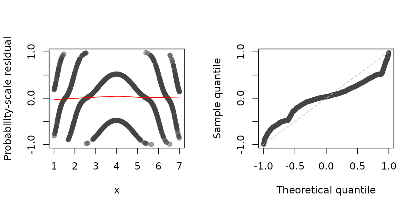

Figure 1: SBS residual plots for the (correctly specified) probit model fit to the df1 data set. Left: Residual-vs-covariate plot with a nonparametric smooth (red curve). Right: Q-Q plot of the residuals.

par(op)

Note: the reference distribution for the SBS residual is the $U\left(-1, 1\right)$ distribution.) As can be seen in the left side of Figure (1), the SBS residuals, which are inherently discrete, often display unusual patterns in diagnostic plots, making them less useful as a diagnostic tool. There is a pattern for each of the $J = 4$ classes!

Similarly, wee can use the resids function to obtain the surrogate residuals. This is illustrated in the following code chunk; and the results are displayed in the figure that follows. (Note: since the surrogate residuals are based on random sampling, we specify the seed via the set.seed function throughout for reproducibility.)

# for reproducibility
set.seed(101)  
sres <- resids(fit.polr)

# Residual-vs-covariate plot and Q-Q plot
op <- par(mfrow = c(1, 2))
plot(sres, what = "covariate", covariate = df1$x, xlab = "x")
plot(sres, what = "qq", distribution = qnorm)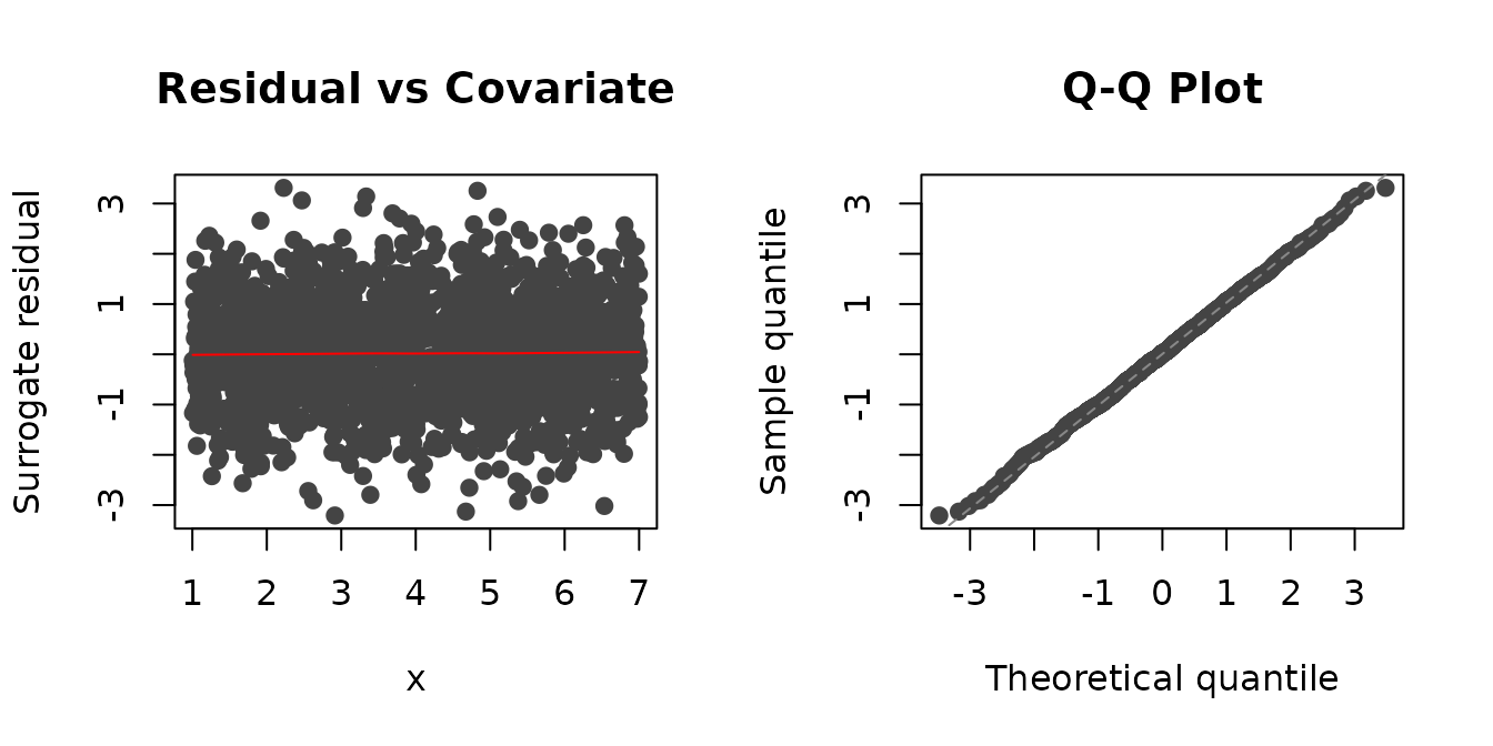

Figure 2: Surrogate residual plots for the (correctly specified) probit model fit to the df1 data set. Left: Residual-vs-covariate plot with a nonparametric smooth (red curve). Right: Q-Q plot of the residuals.

par(op)

The sure package also includes plot methods for the various classes of models listed in Table 1, so you can just give plot the fitted model directly. The benefit of this approach is that the fitted values and reference distribution (used in Q-Q plots) are automatically extracted. For example, to reproduce the Q-Q plot in Figure 2, we could have just used:

# for reproducibility
set.seed(101) 

# same as top right of Figure 1
plot(fit.polr, what = "qq")  

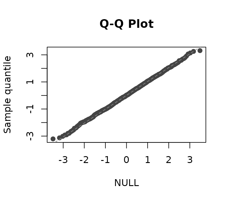
Figure 3: plot option.

Suppose that we did not include the quadratic term in our fitted model. We would expect a residual-vs-$x$ plot to indicate that such a quadratic term is missing. Below we update the previously fitted model by removing the quadratic term, then update the residual-vs-covariate plots (code not shown). The updated residual plots are displayed in Figure 4.

# remove quadratic term
fit.polr <- update(fit.polr, y ~ x) 

set.seed(1055)
op <- par(mfrow = c(1, 2))
plot(fit.polr, what = "covariate", covariate = df1$x, alpha = 0.5,
     xlab = "x", ylab = "Surrogate residual", main = "")

pres <- presid(fit.polr)
plot(x = df1$x, y = pres, col = adjustcolor("#444444", alpha.f = 0.5),
     pch = 19, cex = 1, xlab = "x", ylab = "Probability-scale residual", main = "")
lines(lowess(df1$x, pres), col = "red", lwd = 1.2)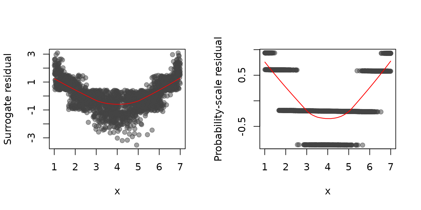

Figure 4: Residual-vs-covariate plots with nonparametric smooths (red curves) for a probit model with a misspecified mean structure fit to the simulated data from model (6). Left: Surrogate residuals. Right: SBS residuals.

par(op) 

The SBS residuals gives some indication of a misspecified mean structure, but this only becomes more clear with increasing $J$, and the plot is still discrete. This is overcome by the surrogate residuals which produces a residual plot not unlike those seen in ordinary linear regression models.

Detecting heteroscedasticty

One issue that often raises concerns in statistical inference is that of heteroscedasticity; that is, when the error term has non constant variance. Heteroscedasticity can bias the statistical inference and lead to improper standard errors, confidence intervals, and $p$-values. Therefore, it is imperative to identify heteroscedacticity whenever present and take appropriate action (e.g., transformations, etc.). In ordinary linear regression, this topic has been covered extensively. For categorical models, on the other hand, not much has been proposed in the literature.

As discussed when introducing surrogate residuals, one of the properties of $R_S$ is that, if the model is specified correctly, then $Var\left(R_S | X\right) = c$, where $c$ is a constant.

For this example, we generated $n = 2000$ observations from the following ordered probit model:

$$Pr\left\{Y \le j\right\} = \Phi\left\{\left(\alpha_j + \beta X\right) / \sigma_X\right\}, \quad j = 1, 2, 3, 4, 5,$$

where $\alpha_1 = -36$, $\alpha_2 = -6$, $\alpha_3 = 34$, $\alpha_4 = 64$, $\beta = -4$, $X \sim U\left(2, 7\right)$, and $\sigma_X = X ^ 2$. Notice how the variability is an increasing function of $X$. These data can be simulated using sim_data(type = "heteroscedastic") (referred to as df2 below).

The following block of code uses the orm function from the popular rms package to fit a probit model to the simulated data. Note: we had to set x = TRUE in the call to orm in order to use the presid function later.

# Simulate heteroscedastic data
set.seed(108)
df2 <- sim_data(n = 2000, type = "heteroscedastic")

# Fit a cumulative link model with probit link
library(rms)  # for orm function
fit.orm <- orm(y ~ x, data = df2, family = "probit", x = TRUE, y = TRUE)

If heteroscedasticity is present, we would expect this to show up in various diagnostic plots, such as a residual-vs-covariate plot. Below we obtain the SBS and surrogate residuals as before and plot them against $X$. The results are displayed in Figure~.

# for reproducibility
set.seed(102)  

op <- par(mfrow = c(1, 2))
plot(resids(fit.orm), what = "covariate", covariate = df2$x, xlab = "x")

pres <- presid(fit.orm)
plot(x = df2$x, y = pres, col = adjustcolor("#444444", alpha.f = 0.25),
     pch = 19, cex = 1, xlab = "x", ylab = "Probability scale residual", main = "")
lines(lowess(df2$x, pres), col = "red", lwd = 1.2)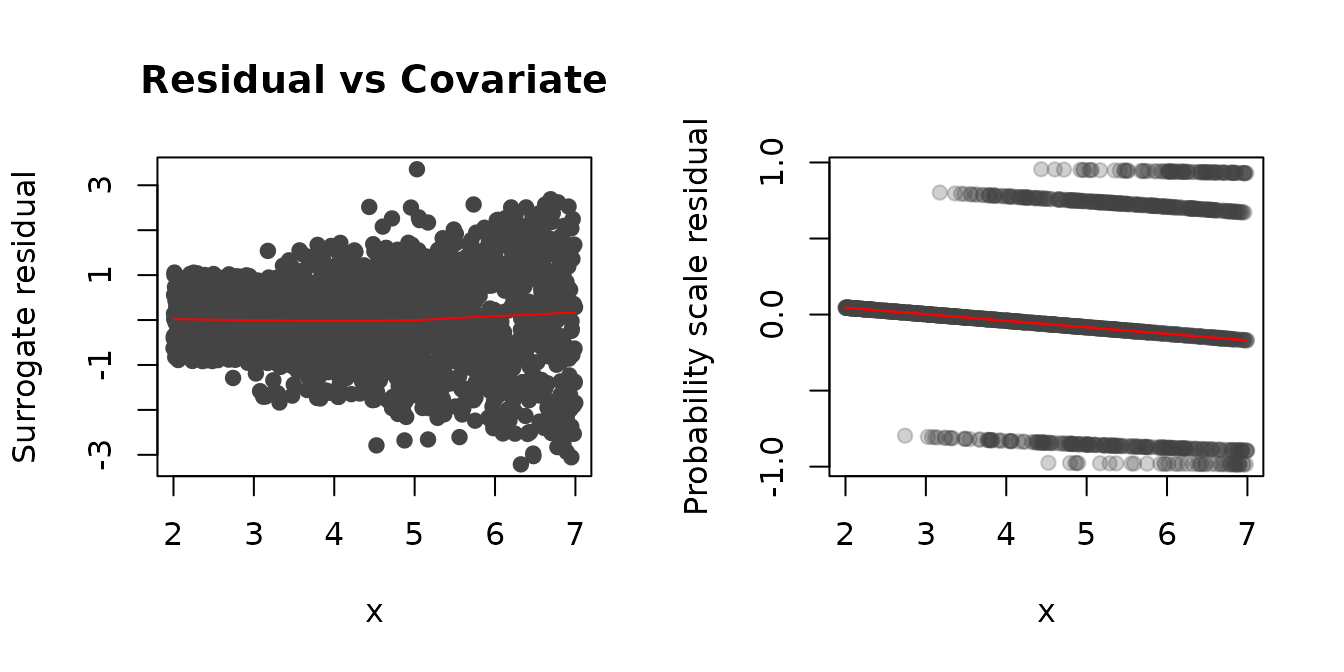

Figure 5: Residual-vs-covariate plots with nonparametric smooths (red curves) for the simulated heteroscedastic data. Left: Surrogate residuals. Right: SBS residuals.

par(op)

In Figure (5), it is clear from the plot of the surrogate residuals (left side of Figure (5)) that the variance increases with $X$, a sign of heteroscedasticity. As a matter of fact, the plot suggests that the true link function has a varying scale parameter, $\sigma = \sigma\left(\boldsymbol{X}\right)$. The plot of the SBS residuals (right side of Figure (5)), on the other hand, gives no indication of an issue with nonconstant variance.

As outlined in section about jittering, the jittering technique is broadly applicable to virtually all parametric and nonparametric models for ordinal responses. To illustrate, the code chunk below uses the VGAM package to fit a vector generalized additive model to the same data using a nonparametric smooth for $x$.

library(VGAM)  # for vgam and vglm functions
fit.vgam <- vgam(y ~ s(x), family = cumulative(link = probitlink, parallel = TRUE),
                 data = df2)

To obtain a surrogate residual using the jittering technique, we can set method = "jitter" in the call to resids or plot. There is also the option jitter.scale which can be set to either "probability", for jittering on the probability scale (the default), or "response", for jittering on the response scale. In the code chunk below, we use the plot method to obtain residual-by-covariate plots using both types of jittering. The results, which are displayed in Figure 6, clearly indicate that the variance increases with increasing $x$.

# for reproducibility
set.seed(103)  

op <- par(mfrow = c(1, 2))
res1 <- resids(fit.vgam, method = "jitter")
plot(res1, what = "covariate", covariate = df2$x, xlab = "x", main = "Probability scale")

res2 <- resids(fit.vgam, method = "jitter", jitter_scale = "response")
plot(res2, what = "covariate", covariate = df2$x, xlab = "x", main = "Response scale")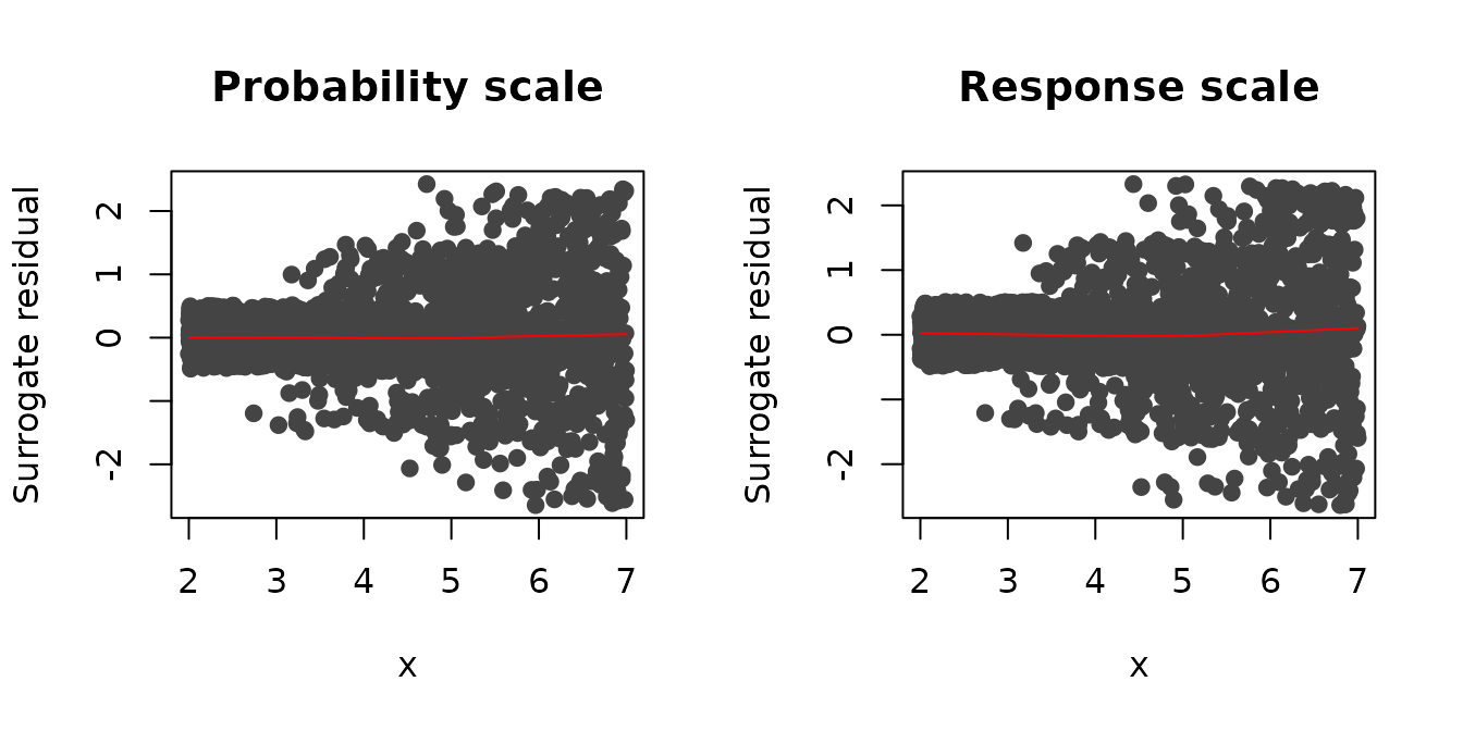

Figure 6: Residual-vs-covariate plots with nonparametric smooths (red curves) from a vector generalized additive model fit to the simulated heteroscedastic data. Left: Jittering on the probability scale (default). Right: Jittering on the response scale.

par(op)

Detecting a misspecified link function

For this example, we simulated $n = 2000$ observations from the following model

$$Pr\left(Y \le j\right) = G\left(\alpha_j - 8 X + X ^ 2\right), \quad j = 1, 2, 3, 4,$$

where $G\left(\cdot\right)$ is the CDF for the Gumbel (max) distribution (see Table 1), $\alpha_1 = -16$, $\alpha_2 = -12$, $\alpha_3 = -8$, $\beta_1 = -8$, $\beta_2 = 1$, and $X \sim U\left(1, 7\right)$. The data can be simulated using sim_data(type = "gumbel") (referred to as df3 below).

Below we fit a model with various link functions. For this model, however, the correct link function to use is the log-log link. From these models, we construct Q-Q plots of the residuals using $R = 100$ bootstrap replicates. From the Q-Q plots in Figure 7, it is clear that the model with the log-log link (which corresponds to Gumbel (max) errors in the latent variable formulation) is the most appropriate, while the other plots indicate deviations from the hypothesized model.

# Simulate Gumbel data
set.seed(977)
df3 <- sim_data(n = 2000, type = "gumbel")

# Fit models with various link functions to the simulated data
fit.probit <- polr(y ~ x + I(x ^ 2), data = df3, method = "probit")
fit.logistic <- polr(y ~ x + I(x ^ 2), data = df3, method = "logistic")
fit.loglog <- polr(y ~ x + I(x ^ 2), data = df3, method = "loglog")  # correct link
fit.cloglog <- polr(y ~ x + I(x ^ 2), data = df3, method = "cloglog")

# Construct Q-Q plots of the surrogate residuals for each model
set.seed(1056)  # for reproducibility
op <- par(mfrow = c(2, 2))
plot(fit.probit, nsim = 100, what = "qq", main = "probit")
plot(fit.logistic, nsim = 100, what = "qq", main = "logistic")
plot(fit.loglog, nsim = 100, what = "qq", main = "log-log (correct)")
plot(fit.cloglog, nsim = 100, what = "qq", main = "cloglog")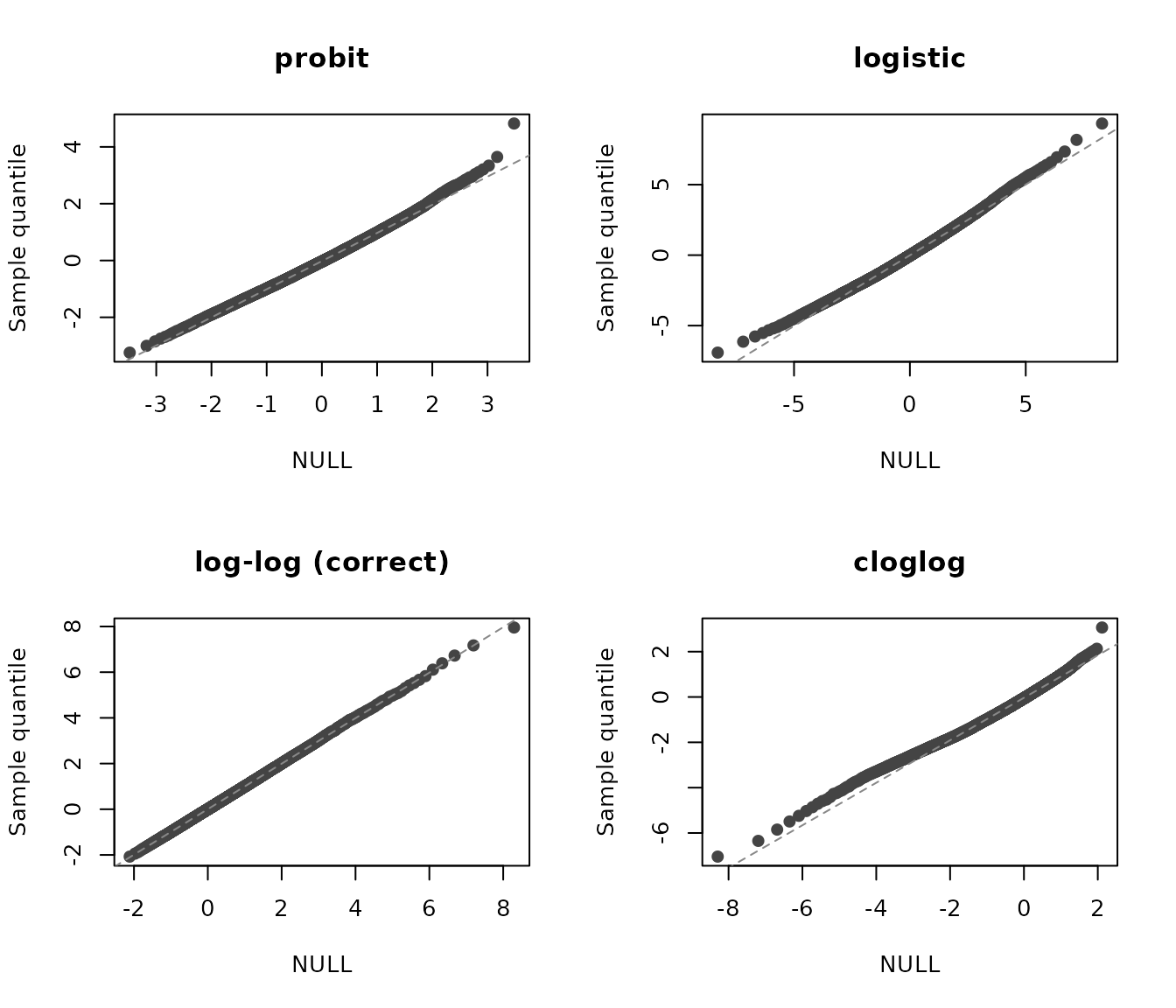

Figure 7: Q-Q plots of the residuals for various cumulative link models fit to simulated data with Gumbel (max) errors. Top left: A model with probit link. Top right: A model with logit link. Bottom left: A model with log-log link (i.e., the correct model). Bottom right: A model with complementary log-log link.

par(op)

Alternatively, we could also use the surrogate residuals to make use of existing distance-based goodness-of-fit (GOF) tests; for example, the Kolmogorov-Smirnov distance. The gof function in sure can be used to produce simulated $p$-values from such tests.

Currently, the gof function supports three goodness-of-fit tests: the Kolmogorov-Smirnov test (test = "ks"), the Anderson-Darling test (test = "ad"), and the Cramer-Von Mises test (test = "cvm"). Below, we use the gof function to simulate $p$-values from the Anderson-Darling test for each of the four models; we also set nsim to 100 to produce smoother plots and reduce the sampling error induced by the surrogate procedure. The plot method is then used to display the empirical distribution function (EDF) of the simulated $p$-values. A good fit would imply uniformly distributed $p$-values; hence, the EDF would be relatively straight with a slope of one. The results, which are displayed in Figure 8, agree with the Q-Q plots from Figure 7 in that the log-log link is the most appropriate for these data. (Note: the plotting method for "gof" objects uses base R graphics; hence, we can use the par function to set various graphical parameters.)

par(mfrow = c(2, 2), mar = c(2, 4, 2, 2) + 0.1)
set.seed(8491)  # for reproducibility
plot(gof(fit.probit, nsim = 100, test = "ad"), main = "")
plot(gof(fit.logistic, nsim = 100, test = "ad"), main = "")
plot(gof(fit.loglog, nsim = 100, test = "ad"), main = "")
plot(gof(fit.cloglog, nsim = 100, test = "ad"), main = "")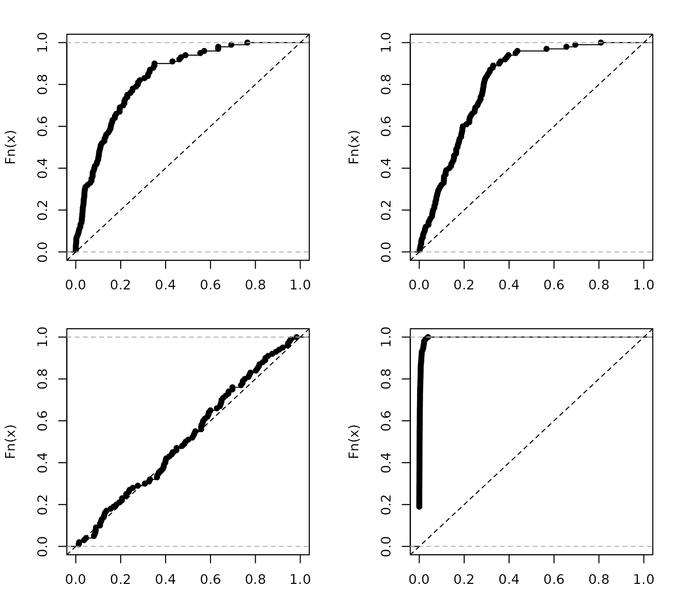

Figure 8: EDFs of the simulated $p$-values from an Anderson-Darling GOF test for various cumulative link models fit to simulated data with gumbel errors. Top left: A model with probit link. Top right: A model with logit link. Bottom left: A model with log-log link (i.e., the correct model). Bottom right: A model with complementary log-log link.

Checking the proportionality assumption

An important feature of the cumulative link model (1) is the proportional odds assumption, which assumes that the mean structure, $f\left(\boldsymbol{X}, \boldsymbol{\beta}\right)$, remains the same for each of the $J$ categories; for the logit case (see row one of Table 1), this is also referred to as the proportional odds assumption. Harrell (2001) suggests computing each observation’s contribution to the first derivative of the log likelihood function with respect to $\boldsymbol{\beta}$, averaging them within each of the $J$ categories, and examining any trends in the residual plots, but these plots can be difficult to interpret. Fortunately, it is relatively straightforward to use the simulated surrogate response values $S$ to check the proportionality assumption.

To illustrate, we generated 2000 observations from each of the following probit models

$$Pr\left(Y \le j\right) = \Phi\left(\alpha_j + \beta_1 X\right), \quad j = 1, 2, 3, \quad \textrm{and} \quad Pr\left(Y \le j\right) = \Phi\left(\alpha_j + \beta_2 X\right), \quad j = 4, 5, 6,$$

where $\alpha_1 = -1.5$, $\alpha_2 = 0$, $\alpha_3 = 1$, $\alpha_4 = 3$, $\beta_1 = 1$, $\beta_2 = 1.5$, and $X \sim U\left(-3, 3\right)$. The data can be simulated using sim_data(n = 4000, type = "proportionality") (referred to as df4 below).

Checking the proportionality assumption here amounts to checking whether or not $\beta_1 - \beta_2 = 0$. As outlined in Liu and Zhang (2017), we can generate surrogates $S_1 \sim N\left(-\beta_1 X, 1\right)$ and $S_2 \sim N\left(-\beta_2 X, 1\right)$, both conditional on $X$. We then define the difference $D = S_2 - S_1$ which, conditional on $X$, follows a $N\left(\left(\beta_1 - \beta_2\right) X, 1\right)$ distribution. If $\beta_1 - \beta_2 = 0$, then $D$ should be independent of $X$. This can be easily checked by plotting $D$ against $X$. Below, we use the surrogate function to generate the surrogate response values directly (as opposed to the residuals) and generate the $D$-vs-$X$ plot shown in Figure 9. It is clear that $\beta_1 - \beta_2 Ne 0$; hence, the proportionality assumption does not hold.

# Simulate proportionality data
set.seed(977)
df4 <- sim_data(n = 4000, type = "proportionality")

# Fit separate models (VGAM should already be loaded)
fit1 <- vglm(y ~ x, data = df4[1:2000, ],
             cumulative(link = probitlink, parallel = TRUE))
fit2 <- update(fit1, data = df4[2001:4000, ])

# Generate surrogate response values
set.seed(8671)  # for reproducibility
s1 <- surrogate(fit1)
s2 <- surrogate(fit2)

library(tinyplot)
tinyplot(D ~ x, data = data.frame(D = s1 - s2, x = df4[1:2000, ]$x),
         type = "p", col = "#444444", pch = 19, cex = 1,
         ylab = "D")
lines(lowess(df4[1:2000, ]$x, s1 - s2), col = "red", lwd = 1.2)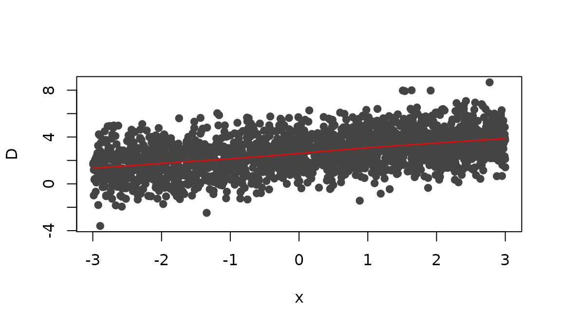

Figure 9: Scatterplot of $D = S_1 - S_2$ vs. $x$ with a nonparametric smooth (red curve).

Detecting interaction effects

A common challenge in model building is determining whether or not there are important interactions between the predictors in the data. Using the surrogate residuals, it is rather straightforward to determine if such an interaction effect is missing from the assumed model.

For illustration, we generated $n = 2000$ observations from the following ordered probit model

$$Pr\left(Y \le j\right) = \Phi\left(\alpha_j + \beta_1 x_1 + \beta_2 x_2 + \beta_3 x_1 x_2\right), \quad j = 1, 2, 3, 4,$$

where $\alpha_1 = -16$, $\alpha_2 = -12$, $\alpha_3 = -8$, $\beta_1 = -5$, $\beta_2 = 3$, $\beta_3 = 10$, $x_1 \sim U\left(1, 7\right)$, and $x_2$ is a factor with levels Treatment and Control. The simulated data can be simulated using sim_data(type = "interaction") (referred to as df5 below). Below, we fit two probit models using the clm function from the ordinal package (which should already be loaded). The first model only corresponds to the simulated control group, while the second model corresponds to the treatment group.

# Simulate interaction data
set.seed(922)
df5 <- sim_data(n = 2000, type = "interaction")

library(ordinal)  # for clm function
fit1 <- clm(y ~ x1, data = df5[df5$x2 == "Control", ], link = "probit")
fit2 <- clm(y ~ x1, data = df5[df5$x2 == "Treatment", ], link = "probit")

If the true model contains an interaction term $x_1 x_2$, but the fitted model does not include it, we can detect this misspecification using the surrogate residuals. We simply plot $R_S$ versus $x_1$ for treatment group, and compare it to the plot of $R_S$ versus $x_1$ for the controls—or better yet, we can just use the surrogate response $S$ instead of $R_S$. The trends in these two plots should be different. Below, we use tinyplot along with the surrogate function to construct such a plot for both fitted models. The results are displayed in Figure~. The plot indicates a negative association between $x_1$ and the outcome within the control group, and a positive association between $x_1$ and the treatment group (i.e., an interaction between $x_1$ and $x_2$).

# for reproducibility
set.seed(1105)  

# surrogate response values
df5$s <- c(surrogate(fit1), surrogate(fit2))

library(tinyplot)
op <- par(mfrow = c(1, 2))

# Control
df5_c <- df5[df5$x2 == "Control", ]
tinyplot(s ~ x1, data = df5_c, type = "p",
         col = adjustcolor("#444444", alpha.f = 0.5), pch = 19, cex = 1,
         ylab = "Surrogate response", xlab = expression(x[1]), main = "Control")
lines(lowess(df5_c$x1, df5_c$s), col = "red", lwd = 1.2)

# Treatment
df5_t <- df5[df5$x2 == "Treatment", ]
tinyplot(s ~ x1, data = df5_t, type = "p",
         col = adjustcolor("#444444", alpha.f = 0.5), pch = 19, cex = 1,
         ylab = "Surrogate response", xlab = expression(x[1]), main = "Treatment")
lines(lowess(df5_t$x1, df5_t$s), col = "red", lwd = 1.2)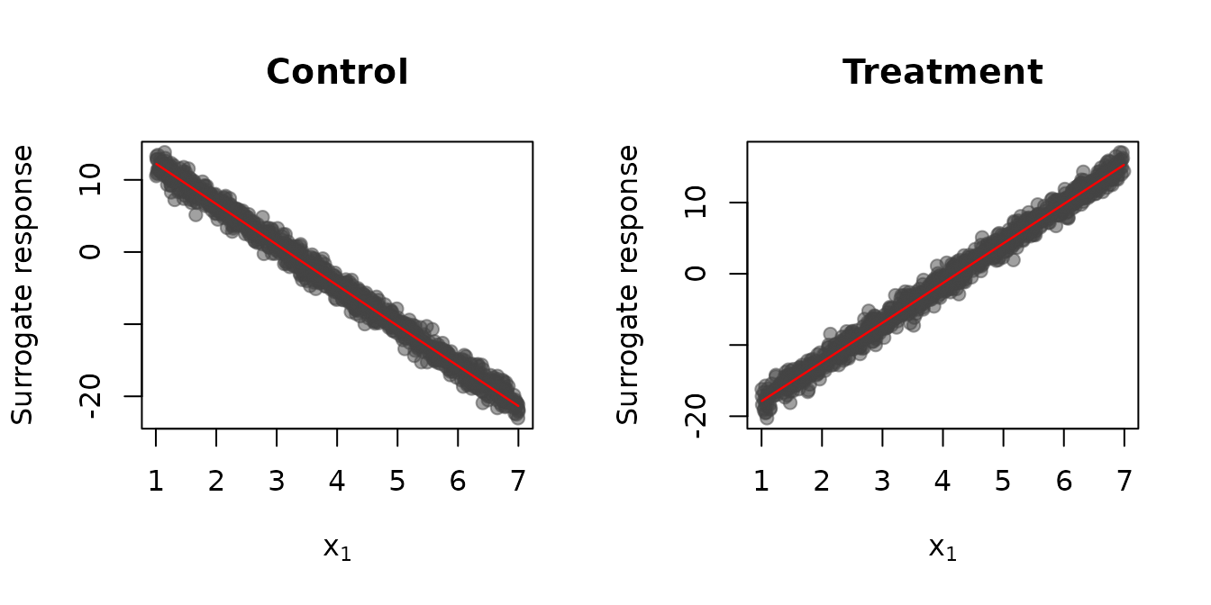

Figure 10: Scatterplot of the surrogate response $S$ versus $x_1$ with a nonparametric smooth (red line). Left: Control group. Right: Treatment group.

par(op)

Bitterness of wine

Randall (1989) performed an experiment on factors determining the bitterness of wine. Two binary treatment factors, temperature and contact (between juice and skin), were controlled while crushing the grapes during wine production. Nine judges each assessed wine from two bottles from each of the four treatment conditions; for a total of $n = 72$. The response is an ordered factor with levels $1 < 2 < 3 < 4 < 5$. The data are available in the ordinal package; see ?ordinal::wine for details.

# load wine data set
data(wine, package = "ordinal")  
wine.clm <- clm(rating ~ temp + contact, data = wine, link = "probit")

Since both of the covariates in this model are binary factors, scatterplots are not appropriate for displaying the residual-by-covariate relationships. Instead, the plot method in sure uses boxplots; a future release is likely to include the additional option for producing nonparametric densities for each level of a factor. The code chunk below uses the plot method to produce some standard residual diagnostic plots. The results are displayed in Figure 11. The Q-Q plot and residual-vs-fitted value plot do not indicate any serious model misspecifications. Furthermore, the boxplots reveal that the medians of the surrogate residuals are very close to zero, and the distribution of the residuals within each level appear to be symmetric and have approximately the same variability (with the exception of a few outliers).

# for reproducibility
set.seed(1225)  

op <- par(mfrow = c(2, 2))
plot(wine.clm, nsim = 10, what = "qq")
plot(wine.clm, nsim = 10, what = "fitted", alpha = 0.5)
plot(wine.clm, nsim = 10, what = "covariate", covariate = wine$temp,
     xlab = "Temperature")
plot(wine.clm, nsim = 10, what = "covariate", covariate = wine$contact,
     xlab = "Contact")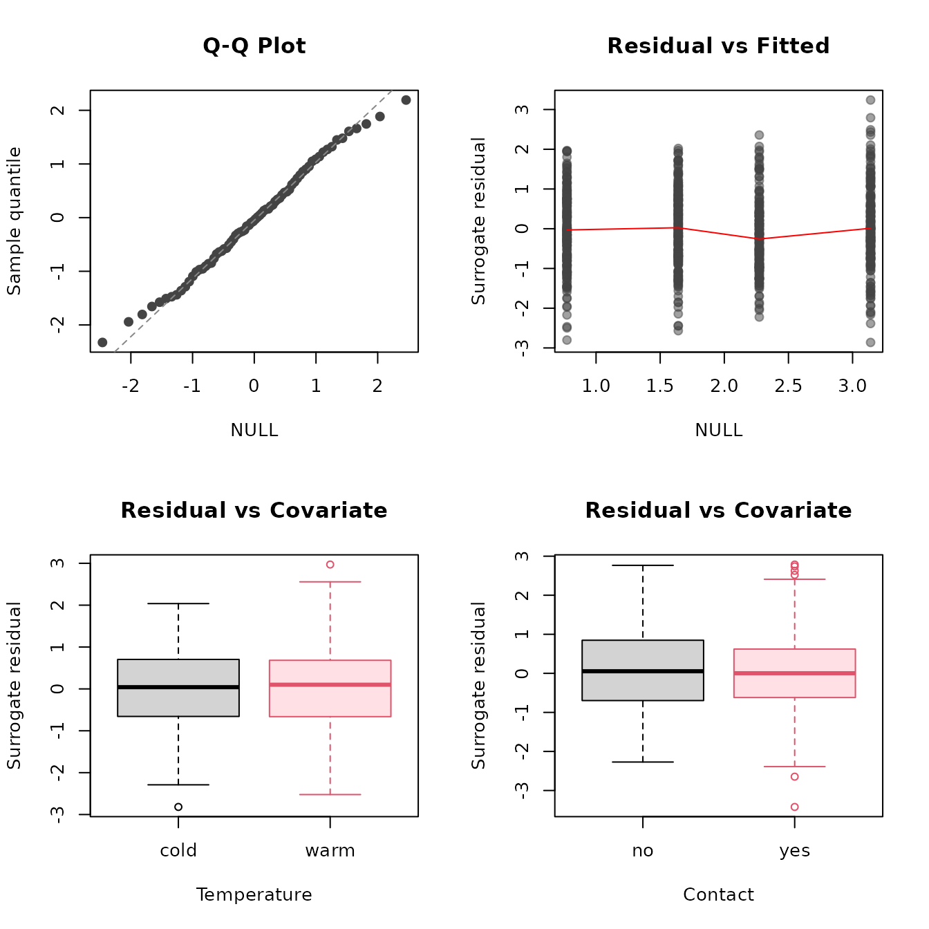

Figure 11: Residual diagnostic plots for the quality of wine example.

par(op)

References

Agresti, Alan. 2010. Analysis of Ordinal Categorical Data. Wiley Series in Probability and Statistics. Wiley.

Christensen, R. H. B. 2015. Ordinal—Regression Models for Ordinal Data. http://www.cran.r-project.org/package=ordinal.

Dupont, Charles, Jeffrey Horner, Chun Li, Qi Liu, and Bryan Shepherd. 2016. PResiduals: Probability-Scale Residuals and Residual Correlations. https://CRAN.R-project.org/package=PResiduals.

Efron, B. 1979. “Bootstrap Methods: Another Look at the Jackknife.” Annals Fo Statistics 7 (1): 1–26. http://dx.doi.org/10.1214/aos/1176344552.

Greenwell, Brandon, Andrew McCarthy, and Brad Boehmke. 2017. Sure: Surrogate Residuals for Ordinal and General Regression Models. https://CRAN.R-project.org/package=sure.

Harrell, Frank E. 2001. Regression Modeling Strategies: With Applications to Linear Models, Logistic Regression, and Survival Analysis. Graduate Texts in Mathematics. Springer.

Harrell Jr, Frank E. 2017. Rms: Regression Modeling Strategies. https://CRAN.R-project.org/package=rms.

Li, Chun, and Bryan E. Shepherd. 2012. “A New Residual for Ordinal Outcomes.” Biometrika 99 (2): 473–80. http://dx.doi.org/10.1093/biomet/asr073.

Liu, Dungang, and Heping Zhang. 2017. “Residuals and Diagnostics for Ordinal Regression Models: A Surrogate Approach.” Journal of the American Statistical Association 0 (ja): 0–0. http://dx.doi.org/10.1080/01621459.2017.1292915.

Liu, Ivy, Bhramar Mukherjee, Thomas Suesse, David Sparrow, and Sung Kyun Park. 2009. “Graphical Diagnostics to Check Model Misspecification for the Proportional Odds Regression Model.” Statistics in Medicine 28 (3): 412–29. http://dx.doi.org/10.1080/01621459.2017.1292915.

Randall, J. H. 1989. “The Analysis of Sensory Data by Generalized Linear Model.” Biometrical Journal 31 (7): 781–93. http://dx.doi.org/10.1002/bimj.4710310703.

Venables, W. N., and B. D. Ripley. 2002. Modern Applied Statistics with s. Fourth. Springer. http://www.stats.ox.ac.uk/pub/MASS4.

Yee, Thomas W. 2017. VGAM: Vector Generalized Linear and Additive Models. https://CRAN.R-project.org/package=VGAM.