GUIDE and CART on scikit-learn’s classification datasets

This notebook compares GuideClassifier with scikit-learn’s DecisionTreeClassifier, which implements CART, on the iris, wine and breast cancer datasets bundled with scikit-learn.

The two methods differ in how they choose splits:

• CART searches every variable and every cutpoint for the split that most reduces impurity. Variables with many distinct values offer more candidate splits, so they win more often, even when they carry no information (see the selection bias notebook).

• GUIDE first picks the split variable with chi-square tests of association between the response and each predictor (plus pairwise interaction tests), then searches only that variable for the best split point.

By default, scikit-learn grows CART trees until the leaves are pure, while GUIDE prunes by 10-fold cross-validation. For a fair comparison we also tune CART’s cost-complexity parameter ccp_alpha by cross-validation.

import matplotlib.pyplot as plt
import numpy as np
import pandas as pd
from sklearn.datasets import load_breast_cancer, load_iris, load_wine
from sklearn.model_selection import GridSearchCV, StratifiedKFold, cross_validate
from sklearn.tree import DecisionTreeClassifier
from sklearn.tree import plot_tree as plot_cart

from guide import GuideClassifier, plot_tree

pd.set_option("display.width", 120)

Iris

plot_tree draws a fitted GUIDE tree with matplotlib. Each internal node shows its split condition; samples that satisfy it go left (“yes”).

iris = load_iris(as_frame=True)
X, y = iris.data, iris.target.map(dict(enumerate(iris.target_names)))

guide = GuideClassifier().fit(X, y)
cart = DecisionTreeClassifier(random_state=0).fit(X, y)

fig, axes = plt.subplots(1, 2, figsize=(15, 5.5))
plot_tree(guide, ax=axes[0])
axes[0].set_title(f"GUIDE, pruned by cross-validation ({guide.get_n_leaves()} leaves)")
plot_cart(cart, feature_names=list(X.columns), class_names=list(cart.classes_), filled=True,
          impurity=False, fontsize=6, ax=axes[1])
axes[1].set_title(f"CART, scikit-learn defaults ({cart.get_n_leaves()} leaves)")
plt.show()

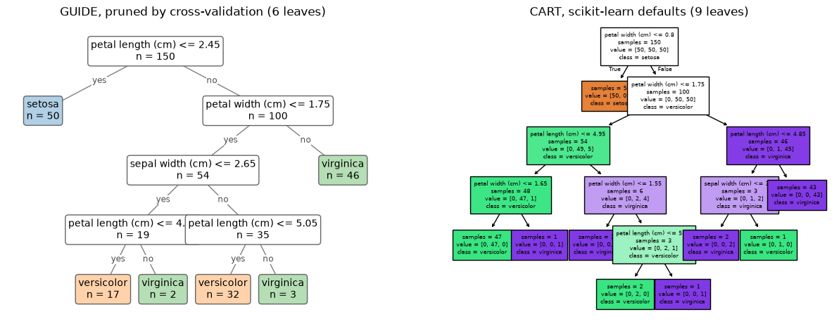
The same tree as text, including the leaf class probabilities and the route taken by missing values:

print(guide.to_text())

guide-rs-0.1-experimental-reference28
1 tree(s), 6 fitted leaves
Tree 1
node 0 (n=150): petal length (cm) <= 2.450000; missing -> no
  node 1 (n=50): class "setosa"; p=[0.9955849889624725, 0.002207505518763797, 0.002207505518763797]
  node 2 (n=100): petal width (cm) <= 1.750000; missing -> no
    node 3 (n=54): sepal width (cm) <= 2.650000; missing -> no
      node 4 (n=19): petal length (cm) <= 4.950000; missing -> no
        node 5 (n=17): class "versicolor"; p=[0.002207505518763797, 0.9371510193481367, 0.06064147513309961]
        node 8 (n=2): class "virginica"; p=[0.002207505518763797, 0.002207505518763797, 0.9955849889624725]
      node 9 (n=35): petal length (cm) <= 5.050000; missing -> no
        node 10 (n=32): class "versicolor"; p=[0.002207505518763797, 0.9955849889624725, 0.002207505518763797]
        node 11 (n=3): class "virginica"; p=[0.002207505518763797, 0.33333333333333337, 0.6644591611479029]
    node 12 (n=46): class "virginica"; p=[0.002207505518763797, 0.02380266820232268, 0.9739898262789137]

Probability quality, ranking and tree size

We report ten-fold cross-validated metrics, with the mean number of leaves and fit time:

• Log loss (lower is better): the average negative log probability given to the true class. It punishes confident mistakes heavily.

• Brier score (lower is better): the squared distance between the predicted probability vector and the observed class, summed over classes (0 to 2).

• AUROC (higher is better): how well the predicted probabilities rank the classes; for iris and wine, each class against the rest, averaged over classes.

• Accuracy (higher is better): the share of samples whose most probable class is correct, shown for reference.

Log loss and the Brier score are proper scoring rules: they are optimized, in expectation, only by the true class probabilities. Accuracy is not. It ignores how confident a prediction is, depends on an arbitrary decision threshold, changes in steps as single samples flip, and can favor a model with badly calibrated probabilities. It also looks deceptively good when one class dominates. Proper scoring rules are almost always the better basis for comparing and tuning classifiers.

“CART, tuned” chooses ccp_alpha by an inner 5-fold grid search on log loss, the closest analog of GUIDE’s built-in pruning. GUIDE’s own pruning minimizes cross-validated misclassification cost, not log loss.

def leaves(model):
    model = getattr(model, "best_estimator_", model)
    return model.get_n_leaves() if hasattr(model, "get_n_leaves") else np.nan


def compare(models, X, y, cv, scoring=None):
    # A dict of scorers gives one column per metric; scikit-learn's negated
    # losses ("neg_...") are reported as losses.
    metrics = scoring if isinstance(scoring, dict) else {"score": scoring}
    rows = []
    for name, model in models.items():
        result = cross_validate(model, X, y, cv=cv, scoring=metrics, return_estimator=True)
        row = {"model": name}
        for metric, scorer in metrics.items():
            loss = getattr(scorer, "negated", False) or str(scorer).startswith("neg_")
            sign = -1 if loss else 1
            row[metric] = sign * result[f"test_{metric}"].mean()
            if len(metrics) == 1:
                row["sd"] = result[f"test_{metric}"].std()
        row["leaves"] = np.mean([leaves(e) for e in result["estimator"]])
        row["fit seconds"] = result["fit_time"].mean()
        rows.append(row)
    return pd.DataFrame(rows).set_index("model").round(3)


def cart_tuned():
    grid = {"ccp_alpha": np.r_[0, np.logspace(-4, -1, 12)]}
    return GridSearchCV(DecisionTreeClassifier(random_state=0), grid, cv=5, scoring="neg_log_loss")


models = {
    "GUIDE": GuideClassifier(),
    "CART, defaults": DecisionTreeClassifier(random_state=0),
    "CART, tuned": cart_tuned(),
}
def brier(model, X, y):
    # Squared error of the probability vector, summed over classes (0 to 2),
    # for binary and multiclass data alike; negated like scikit-learn's losses.
    observed = np.asarray(y)[:, None] == model.classes_
    return -np.mean(((model.predict_proba(X) - observed) ** 2).sum(axis=1))


brier.negated = True
metrics = {"log loss": "neg_log_loss", "Brier": brier, "AUROC": "roc_auc_ovr", "accuracy": "accuracy"}
def named(bunch):
    return bunch.data, bunch.target.map(dict(enumerate(bunch.target_names)))


datasets = {
    "iris": (X, y),
    "wine": named(load_wine(as_frame=True)),
    "breast cancer": named(load_breast_cancer(as_frame=True)),
}
cv = StratifiedKFold(10, shuffle=True, random_state=0)
pd.concat({name: compare(models, *data, cv, metrics) for name, data in datasets.items()})

		log loss	Brier	AUROC	accuracy	leaves	fit seconds
	model
iris	GUIDE	0.287	0.128	0.962	0.933	3.9	0.001
	CART, defaults	2.163	0.120	0.955	0.940	8.6	0.001
	CART, tuned	0.475	0.146	0.958	0.920	3.3	0.093
wine	GUIDE	0.487	0.176	0.936	0.905	6.4	0.003
	CART, defaults	4.264	0.237	0.911	0.882	9.4	0.001
	CART, tuned	1.052	0.386	0.858	0.774	3.1	0.107
breast cancer	GUIDE	0.217	0.106	0.954	0.942	6.4	0.023
	CART, defaults	2.789	0.155	0.917	0.923	21.0	0.003
	CART, tuned	0.323	0.177	0.895	0.900	2.5	0.242

GUIDE has the lowest log loss and the highest AUROC on all three datasets, and the lowest Brier score on wine and breast cancer. On iris default CART’s Brier score is slightly lower (0.120 against 0.128).

Accuracy would tell a different story on iris: default CART classifies slightly more flowers correctly than GUIDE (0.940 against 0.933), although its probabilities are far worse.

Default CART grows pure leaves, so it predicts probabilities of exactly 0 and 1, and each confident mistake costs about 36 in log loss after scikit-learn clips the probability. Its log loss is therefore 7 to 13 times GUIDE’s, even on iris, where its Brier score is the lower one. Tuning CART on log loss avoids that by pruning hard, to about three leaves, but its Brier score is then worse than default CART’s on all three datasets, and its AUROC on wine and breast cancer. GUIDE never predicts a probability of exactly 0: classes absent from a leaf get a small probability from the class priors (GUIDE’s zero-posterior correction), which keeps its log loss finite.

On the breast cancer data GUIDE is slower than default CART but faster than CART tuned by grid search; its cross-validation folds run in parallel. When an interaction test selects a pair of predictors, GUIDE scores each split on the first by the best split on the second in each child, a one-level lookahead; interactions=False skips the interaction tests and the lookahead.

Breast cancer trees

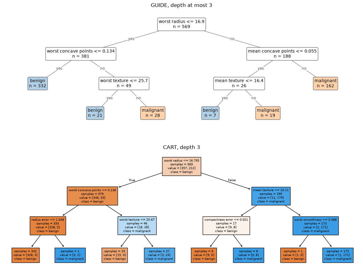
GUIDE’s variable selection and CART’s exhaustive search can pick different root variables even when both trees predict well. Restricting both to depth 3 for display:

Xb, yb = datasets["breast cancer"]
guide_b = GuideClassifier(max_depth=3).fit(Xb, yb)
cart_b = DecisionTreeClassifier(max_depth=3, random_state=0).fit(Xb, yb)

fig, axes = plt.subplots(2, 1, figsize=(15, 11))
plot_tree(guide_b, ax=axes[0])
axes[0].set_title("GUIDE, depth at most 3")
plot_cart(cart_b, feature_names=list(Xb.columns), class_names=list(cart_b.classes_), filled=True,
          impurity=False, fontsize=7, ax=axes[1])
axes[1].set_title("CART, depth 3")
plt.show()

Forests and boosted ensembles of GUIDE trees are compared with scikit-learn’s in the ensembles notebook.