GUIDE and CART regression trees on the diabetes data

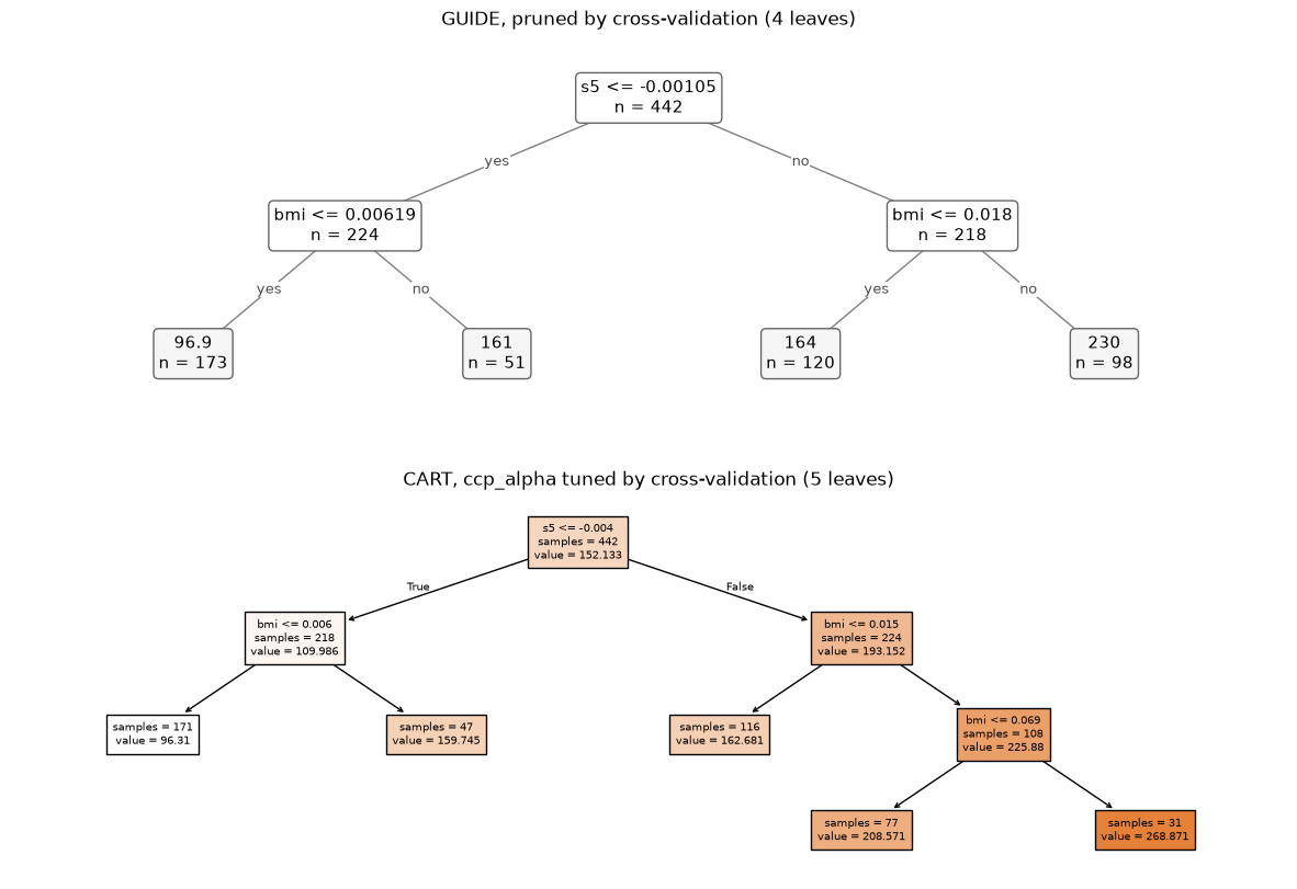
This notebook compares GuideRegressor with scikit-learn’s DecisionTreeRegressor (CART) on the diabetes dataset bundled with scikit-learn: ten baseline variables for 442 patients and a measure of disease progression one year later.

Besides piecewise-constant trees like CART’s, GUIDE can fit a linear model in each leaf, which often gives a smaller tree that fits as well, and it can fit quantile trees.

import matplotlib.pyplot as plt
import numpy as np
import pandas as pd
from sklearn.datasets import load_diabetes
from sklearn.model_selection import GridSearchCV, KFold, cross_validate, train_test_split
from sklearn.tree import DecisionTreeRegressor
from sklearn.tree import plot_tree as plot_cart

from guide import GuideRegressor, plot_tree

X, y = load_diabetes(return_X_y=True, as_frame=True)
X.head()

	age	sex	bmi	bp	s1	s2	s3	s4	s5	s6
0	0.038076	0.050680	0.061696	0.021872	-0.044223	-0.034821	-0.043401	-0.002592	0.019907	-0.017646
1	-0.001882	-0.044642	-0.051474	-0.026328	-0.008449	-0.019163	0.074412	-0.039493	-0.068332	-0.092204
2	0.085299	0.050680	0.044451	-0.005670	-0.045599	-0.034194	-0.032356	-0.002592	0.002861	-0.025930
3	-0.089063	-0.044642	-0.011595	-0.036656	0.012191	0.024991	-0.036038	0.034309	0.022688	-0.009362
4	0.005383	-0.044642	-0.036385	0.021872	0.003935	0.015596	0.008142	-0.002592	-0.031988	-0.046641

Piecewise-constant trees

guide = GuideRegressor().fit(X, y)
cart = GridSearchCV(DecisionTreeRegressor(random_state=0),
                    {"ccp_alpha": np.r_[0, np.logspace(0, 3, 13)]}, cv=5).fit(X, y)

fig, axes = plt.subplots(2, 1, figsize=(15, 10))
plot_tree(guide, ax=axes[0])
axes[0].set_title(f"GUIDE, pruned by cross-validation ({guide.get_n_leaves()} leaves)")
plot_cart(cart.best_estimator_, feature_names=list(X.columns), filled=True, impurity=False,
          fontsize=7, ax=axes[1])
axes[1].set_title(f"CART, ccp_alpha tuned by cross-validation "
                  f"({cart.best_estimator_.get_n_leaves()} leaves)")
plt.show()

Linear leaves

With node_model="linear", each leaf fits a least-squares regression. feature_roles controls which variables split and which enter the leaf models; by default every numeric variable can do both.

On these data, cross-validation prunes the linear-leaf tree back to its root: progression is close to linear in the predictors, so a single multiple regression beats any split.

linear = GuideRegressor(node_model="linear").fit(X, y)
print(f"leaves after pruning: {linear.get_n_leaves()}")

leaves after pruning: 1

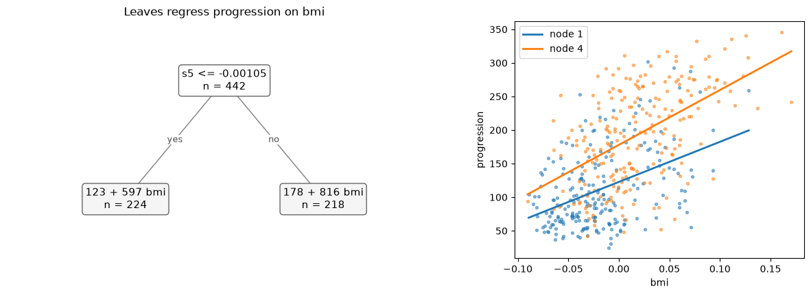
Roles also allow simpler models that are easy to plot. Below, bmi is the only regressor in each leaf and the remaining variables only split, giving a piecewise simple linear regression on bmi. plot_tree shows each leaf’s fitted line:

roles = {name: "split" for name in X.columns} | {"bmi": "fit"}
simple = GuideRegressor(node_model="linear", feature_roles=roles, max_depth=2).fit(X, y)

fig, axes = plt.subplots(1, 2, figsize=(15, 4.5), gridspec_kw={"width_ratios": [3, 2]})
plot_tree(simple, ax=axes[0])
axes[0].set_title("Leaves regress progression on bmi")
leaf = simple.apply(X)
for i, node in enumerate(np.unique(leaf)):
    rows = leaf == node
    axes[1].scatter(X.bmi[rows], y[rows], s=8, alpha=0.5, color=f"C{i}")
    order = np.argsort(X.bmi[rows].to_numpy())
    axes[1].plot(X.bmi[rows].to_numpy()[order], simple.predict(X[rows])[order], color=f"C{i}",
                 lw=2, label=f"node {node}")
axes[1].set(xlabel="bmi", ylabel="progression")
axes[1].legend()
plt.show()

Predictive performance and tree size

Ten-fold cross-validated R², mean leaves and mean fit time. The tuned CART chooses ccp_alpha by an inner 5-fold grid search.

def leaves(model):
    model = getattr(model, "best_estimator_", model)
    return model.get_n_leaves() if hasattr(model, "get_n_leaves") else np.nan


def compare(models, X, y, cv, scoring=None):
    # A dict of scorers gives one column per metric; scikit-learn's negated
    # losses ("neg_...") are reported as losses.
    metrics = scoring if isinstance(scoring, dict) else {"score": scoring}
    rows = []
    for name, model in models.items():
        result = cross_validate(model, X, y, cv=cv, scoring=metrics, return_estimator=True)
        row = {"model": name}
        for metric, scorer in metrics.items():
            loss = getattr(scorer, "negated", False) or str(scorer).startswith("neg_")
            sign = -1 if loss else 1
            row[metric] = sign * result[f"test_{metric}"].mean()
            if len(metrics) == 1:
                row["sd"] = result[f"test_{metric}"].std()
        row["leaves"] = np.mean([leaves(e) for e in result["estimator"]])
        row["fit seconds"] = result["fit_time"].mean()
        rows.append(row)
    return pd.DataFrame(rows).set_index("model").round(3)


models = {
    "GUIDE, constant leaves": GuideRegressor(),
    "GUIDE, linear leaves": GuideRegressor(node_model="linear"),
    "CART, defaults": DecisionTreeRegressor(random_state=0),
    "CART, tuned": GridSearchCV(DecisionTreeRegressor(random_state=0),
                                {"ccp_alpha": np.r_[0, np.logspace(0, 3, 13)]}, cv=5),
}
compare(models, X, y, KFold(10, shuffle=True, random_state=0))

	score	sd	leaves	fit seconds
model
GUIDE, constant leaves	0.350	0.177	5.2	0.018
GUIDE, linear leaves	0.477	0.114	1.1	0.095
CART, defaults	-0.209	0.228	388.6	0.001
CART, tuned	0.335	0.136	5.1	0.121

The single linear model (GUIDE with linear leaves, pruned to one node) has the highest R². Among piecewise-constant trees, GUIDE and tuned CART are close, while the unpruned CART tree overfits badly (negative R²).

Quantile trees

loss="quantile" fits a tree to a conditional quantile. Trees for the 10% and 90% quantiles give an 80% prediction interval; its coverage on held-out data should be near 80%. (scikit-learn’s DecisionTreeRegressor has no quantile criterion.)

X_train, X_test, y_train, y_test = train_test_split(X, y, test_size=0.3, random_state=0)
lower = GuideRegressor(loss="quantile", quantile=0.1).fit(X_train, y_train)
upper = GuideRegressor(loss="quantile", quantile=0.9).fit(X_train, y_train)
lo, hi = lower.predict(X_test), upper.predict(X_test)
print(f"coverage: {np.mean((y_test >= lo) & (y_test <= hi)):.2f}, "
      f"mean width: {np.mean(hi - lo):.0f}")

coverage: 0.78, mean width: 163

Bagged, random-forest and boosted ensembles of GUIDE trees are compared with scikit-learn’s in the ensembles notebook.