Variable selection bias and importance scores

Exhaustive-search trees such as CART favor variables with many distinct values: such a variable offers more cutpoints, so by chance alone one of them is more likely to reduce impurity. GUIDE avoids this bias by choosing the split variable with chi-square tests, whose p-values put variables with different numbers of values on a common scale.

This matters most for interpretation: a tree’s split variables, and importance scores built from them, can point to noise. This notebook shows the effect with a null simulation and then compares importance scores on the diabetes data with added noise variables.

import json

import matplotlib.pyplot as plt
import numpy as np
import pandas as pd
from scipy.stats import chisquare
from sklearn.datasets import load_diabetes
from sklearn.ensemble import RandomForestRegressor
from sklearn.inspection import permutation_importance
from sklearn.model_selection import train_test_split
from sklearn.tree import DecisionTreeRegressor

from guide import GuideRegressor, importance

A null simulation

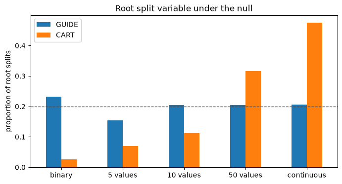
Five predictors, all independent of the response, differ only in their number of distinct values: 2, 5, 10, 50 and continuous. In each of 500 replications we fit a single split (a stump) with each method and record the variable it splits on. With no bias, each variable should be chosen about 20% of the time.

rng = np.random.default_rng(0)
values = {"binary": 2, "5 values": 5, "10 values": 10, "50 values": 50, "continuous": None}
n, reps = 200, 500
chosen = {"GUIDE": [], "CART": []}
for _ in range(reps):
    X = pd.DataFrame({
        name: rng.normal(size=n) if k is None else rng.integers(0, k, n).astype(float)
        for name, k in values.items()
    })
    y = rng.normal(size=n)
    guide = GuideRegressor(max_depth=1, pruning="none", min_gain=0).fit(X, y)
    root = json.loads(guide.to_json())["trees"][0]["root"]
    chosen["GUIDE"].append(X.columns[root["split"]["feature"]])
    cart = DecisionTreeRegressor(max_depth=1).fit(X, y)
    chosen["CART"].append(X.columns[cart.tree_.feature[0]])

counts = pd.DataFrame({m: pd.Series(c).value_counts().reindex(list(values), fill_value=0)
                       for m, c in chosen.items()})
counts / reps

	GUIDE	CART
binary	0.232	0.026
5 values	0.154	0.070
10 values	0.204	0.112
50 values	0.204	0.316
continuous	0.206	0.476

ax = (counts / reps).plot.bar(figsize=(8, 4), rot=0)
ax.axhline(0.2, color="0.3", ls="--", lw=1)
ax.set(ylabel="proportion of root splits", title="Root split variable under the null")
plt.show()
for method in counts:
    print(f"{method}: chi-square test of uniform selection, p = {chisquare(counts[method]).pvalue:.3g}")

GUIDE: chi-square test of uniform selection, p = 0.0908
CART: chi-square test of uniform selection, p = 6.12e-77

CART almost always splits on the continuous or 50-value variable and rarely on the binary one. GUIDE’s choices are consistent with uniform selection.

Importance scores with noise variables

Next, the diabetes data plus three noise variables: a continuous one, a binary one, and a 40-level categorical “clinic” code. We compare:

• GUIDE importance (guide.importance, Loh and Zhou 2021): scores from GUIDE’s selection statistics, adjusted by their mean under permutations of the response, with a threshold separating important from unimportant variables.

• Random forest impurity importance (feature_importances_), which inherits CART’s selection bias.

• Permutation importance of the random forest on a held-out 30% of the data, scikit-learn’s recommended alternative to impurity importance.

X, y = load_diabetes(return_X_y=True, as_frame=True)
rng = np.random.default_rng(1)
X["noise continuous"] = rng.normal(size=len(X))
X["noise binary"] = rng.integers(0, 2, len(X)).astype(float)
clinic = rng.integers(0, 40, len(X))
X_guide = X.assign(clinic=pd.Categorical(clinic.astype(str)))  # GUIDE: categorical
X_sklearn = X.assign(clinic=clinic.astype(float))  # scikit-learn: integer codes

report = importance(GuideRegressor(), X_guide, y)
guide_scores = pd.DataFrame(report["scores"]).set_index("feature")

X_train, X_test, y_train, y_test = train_test_split(X_sklearn, y, test_size=0.3, random_state=0)
forest = RandomForestRegressor(n_estimators=300, random_state=0).fit(X_train, y_train)
permuted = permutation_importance(forest, X_test, y_test, n_repeats=20, random_state=0)

table = pd.DataFrame({
    "GUIDE adjusted": guide_scores["adjusted_score"],
    "GUIDE group": guide_scores["group"],
    "RF impurity": pd.Series(forest.feature_importances_, X_sklearn.columns),
    "RF permutation": pd.Series(permuted.importances_mean, X_sklearn.columns),
})
ranks = table[["GUIDE adjusted", "RF impurity", "RF permutation"]].rank(ascending=False)
table.join(ranks.add_suffix(" rank").astype(int)).sort_values("GUIDE adjusted", ascending=False).round(3)

	GUIDE adjusted	GUIDE group	RF impurity	RF permutation	GUIDE adjusted rank	RF impurity rank	RF permutation rank
s5	19.786	highly_important	0.290	0.177	1	2	1
bmi	17.871	highly_important	0.292	0.160	2	1	2
bp	11.916	highly_important	0.087	0.037	3	3	3
s4	9.628	highly_important	0.024	-0.007	4	11	11
s6	9.133	highly_important	0.044	0.004	5	6	6
s3	8.835	highly_important	0.054	-0.015	6	4	13
noise binary	2.948	unimportant	0.008	0.009	7	12	4
s1	2.736	unimportant	0.034	-0.002	8	10	9
s2	2.375	unimportant	0.038	-0.001	9	8	8
age	2.257	unimportant	0.037	0.004	10	9	5
sex	1.876	unimportant	0.007	0.002	11	13	7
noise continuous	1.739	unimportant	0.047	-0.006	12	5	10
clinic	1.265	unimportant	0.038	-0.014	13	7	12

GUIDE places all three noise variables in its unimportant group. The random forest’s impurity importance ranks the continuous noise and the 40-level clinic code above several real variables, while the binary noise variable, with a single possible cutpoint, ranks near the bottom: the same bias as in the simulation.

Held-out permutation importance has no such bias, but beyond the three strongest variables its values are small and noisy; here the binary noise variable ranks fourth by chance.

Boosting

Gradient boosting fits hundreds of trees to the gradients of the loss, and split counts or gain summed over those trees are a common importance measure. GuideBoostingRegressor (experimental) chooses each split variable with GUIDE’s tests on the signs of the negative gradients, then the split point by the usual second-order gain. The same null simulation, with 50 boosting rounds of depth-3 trees, compares the share of all splits that land on each pure-noise predictor with scikit-learn’s GradientBoostingRegressor:

from sklearn.ensemble import GradientBoostingRegressor

from guide import GuideBoostingRegressor


def guide_split_counts(model, p):
    counts = np.zeros(p)
    def walk(node):
        if node.get("split"):
            counts[node["split"]["feature"]] += 1
            walk(node["left"])
            walk(node["right"])
    for tree in json.loads(model.to_json())["trees"]:
        walk(tree["root"])
    return counts


def sklearn_split_counts(model, p):
    counts = np.zeros(p)
    for tree in model.estimators_.ravel():
        features = tree.tree_.feature
        counts += np.bincount(features[features >= 0], minlength=p)
    return counts


names = list(values)
boost_guide, boost_cart = np.zeros(len(names)), np.zeros(len(names))
rng = np.random.default_rng(100)
for _ in range(20):
    X = pd.DataFrame({
        name: rng.normal(size=n) if k is None else rng.integers(0, k, n).astype(float)
        for name, k in values.items()
    })
    y = rng.normal(size=n)
    boost_guide += guide_split_counts(GuideBoostingRegressor(n_estimators=50).fit(X, y), len(names))
    boost_cart += sklearn_split_counts(
        GradientBoostingRegressor(n_estimators=50, max_depth=3, random_state=0).fit(X, y), len(names))
pd.DataFrame({"GUIDE boosting": boost_guide / boost_guide.sum(),
              "scikit-learn boosting": boost_cart / boost_cart.sum()}, index=names).round(3)

	GUIDE boosting	scikit-learn boosting
binary	0.140	0.042
5 values	0.198	0.102
10 values	0.200	0.160
50 values	0.248	0.266
continuous	0.214	0.431

scikit-learn’s boosted trees split ten times as often on the continuous noise variable as on the binary one (43% of all splits against 4%), so split-count and gain importance would rank pure noise by its number of distinct values. GUIDE boosting spreads its splits much more evenly. The binary variable’s share is somewhat lower because it can split only once along any branch, not because it is selected less often.